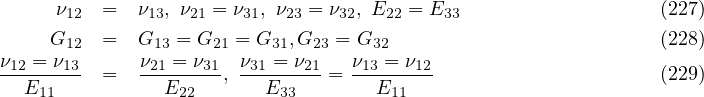
Orthotropic damage model with fixed crack orientations for composites

1.7 Orthotropic damage model with fixed crack orientations for composites - CompDamMat

The model is designed for transversely isotropic elastic material defined by five elastic material constants. Typical example is a carbon fiber tow. Axis 1 represents the material principal direction. The orthotropic material constants are defined as

ν12 = ν13, ν21 = ν31, ν23 = ν32, E22 = E33 (227) G12 = G13 = G21 = G31,G23 = G32 (228) ν12 = ν13 ν21 = ν31 ν31 = ν21 ν13 = ν12 ---E11-- = --E22---,---E33-- = --E11--- (229)

Material orientation on a finite element can be specified with lcs optional parameter. If unspecified, material orientation is the same as the global coordinate system. lcs array contains six numbers, where the first three numbers represent a directional vector of the local x-axis, and the next three numbers represent a directional vector of the local y-axis with the reference to the global coordinate system. The composite material is extended to 1D and is also suitable for beams and trusses. In such particular case, the lcs has no effect and the 1D element orientation is aligned with the global xx component.

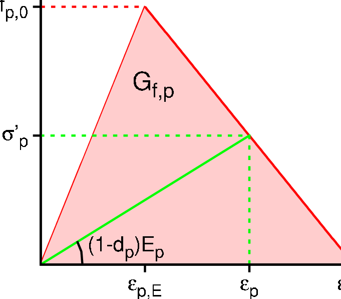
The index p, p ∈{11,22,33,23,31,12} symbolizes six components of stress or strain vectors. The linear softening occurs after reaching a critical stress f_p,0, see Fig. 10. Orientation of cracks is assumed to be orthogonal and aligned with an orientation of material axes [3, pp.236]. The transverse isotropy is generally lost upon fracture, material becomes orthotropic and six damage parameters d_p are introduced.

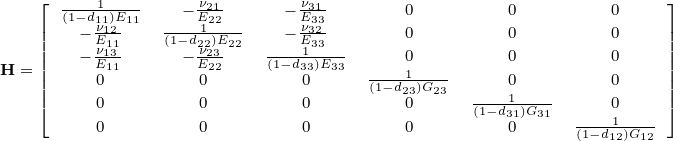
Figure 10: Implemented stress-strain evolution with damage for 1D case. Tension and compression are separated, but sharing the same damage parameter.

The compliance material matrix H, in the secant form and including damage parameters, reads

⌊ (1-d111)E11- - νE2122- -Eν3313 0 0 0 ⌋ || - νE1211 (1-d122)E22- -Eν3323 0 0 0 || ||| - νE1311 - νE2322- (1-d313)E33 0 0 0 ||| H =|| 0 0 0 (1-d213)G23 0 0 || |⌈ 0 0 0 0 (1-d131)G31 0 |⌉ 0 0 0 0 0 (1-d112)G12

(230)

Damage occurs when any out of six stress tensor components exceeds a given strength f_p,0

|σp| ≥ |fp,0|

(231)

Positive and negative ultimate strengths can be generally different but share the same damage variable. At the point of damage initiation, see Fig. 10, one evaluates ε_p,E and characteristic element length l_p, generally different for each damage mode. Given the fracture energy G_F,p, the maximum strain at zero stress ε_p,0 is computed

ε = ε + 2GF,p (232) p,0 p,E fp,0lp

The point of damage initiation is never reached exactly, one needs to interpolate between the previous equilibrated step and current step to achieve objectivity.

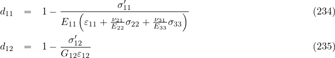
The evolution of damage d_p is based on the evolution of corresponding strain ε_p. A maximum achieved strain is stored in the variable κ_p. If ε_p > κ_p the damage may grow so the corresponding damage variable d_p may increase. Desired stress σ′_p is evaluated from the actual strain ε_p

′ εp,0 - εp σp = fp,0ε----ε--- (233) p,0 p,E

and the calculation of damage variables d_p stems from Eq. 230, for example

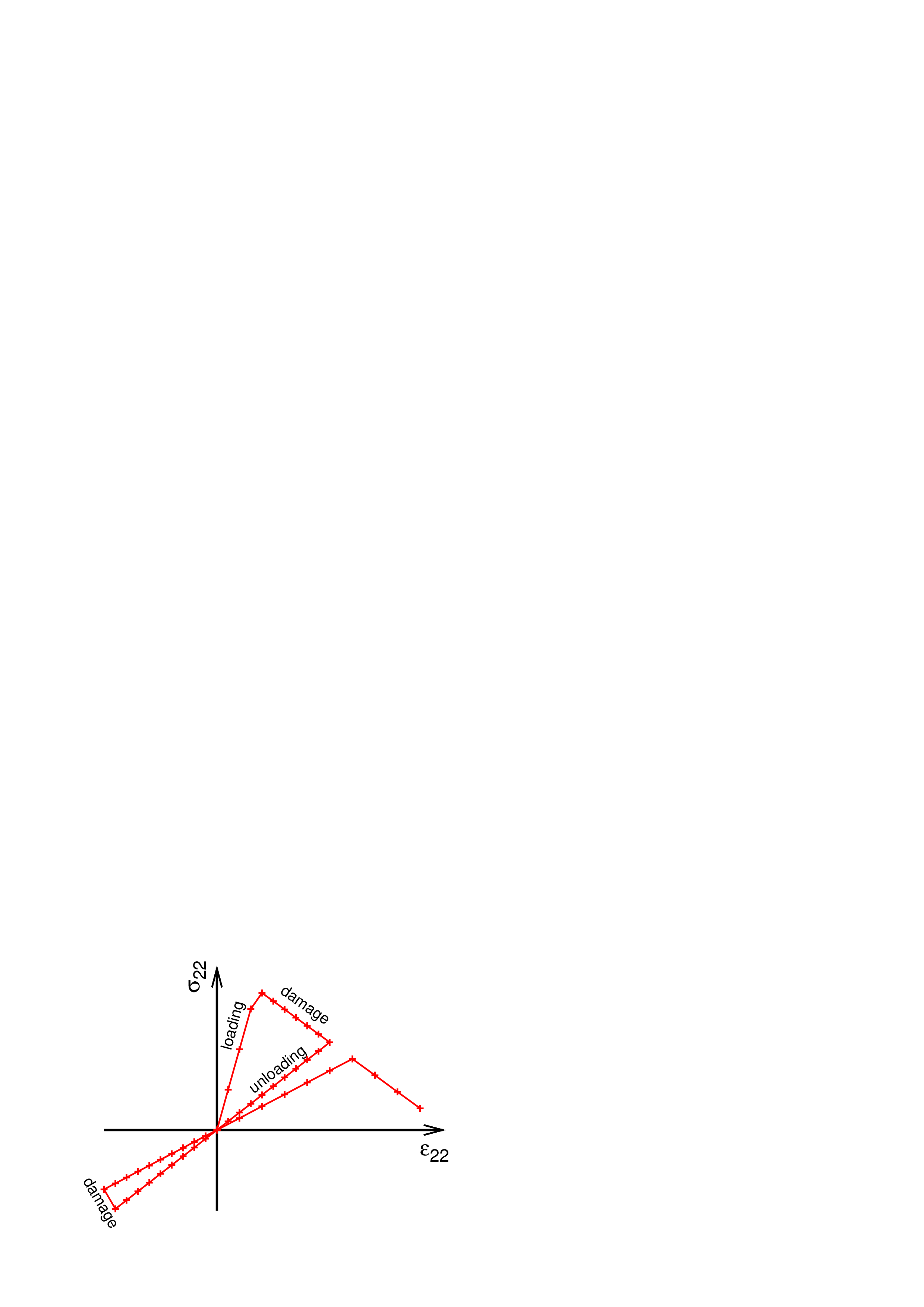
-----------σ′11------------ d11 = 1 - ( -ν21 -ν31 ) (234) E11 ε11 + E22σ22 + E33σ33 -σ′12-- d12 = 1 - G12ε12 (235)

Damage is always controled not to decrease. Fig. 11 shows a typical performance for this damage model in one direction.

The damage initiation is based on a trial stress. It becomes necessary for higher precision to skip a few first iteration, typically 5, and then to introduce damage. A parameter afterIter is designed for this purpose and MinIter forces a solver always to proceed certain amount of iterations.

allowSnapBack skips the checking of sufficient fracture energy for each direction. If not specified, all directions are checked to prevent snap-back which dissipates incorrect amount of energy.

Figure 11: Typical loading/unloading material performance for homogenized stress and strain in the direction ‘2’. Note that one damage parameter is common for both tension and compression.


Description	Orthotropic damage model with fixed crack orientations for composites

Record Format	CompDamMat num(in) # d(rn) # Exx(rn) # EyyEzz(rn) # nuxynuxz(rn) # nuyz(rn) # GxyGxz(rn) # Tension_f0_Gf(ra) # Compres_f0_Gf(ra) # [afterIter(in) #] [allowSnapBack(() #ia)]
Parameters	- num material model number
	- d material density
	- Exx Young’s modulus for principal direction xx
	- EyyEzz Young’s modulus in orthogonal directions to the principal direction xx
	- nuxynuxz Poisson’s ratio in xy and xz directions
	- nuyz Poisson’s ratio in yz direction
	- GxyGxz shear modulus in xy and xz directions
	- Tension_f0_Gf array with six pairs of positive numbers. Each pair describes maximum stress in tension and fracture energy for each direction (xx, yy, zz, yz, zx, xy)
	- Compres_f0_Gf array with six pairs of numbers. Each pair describes maximum stress in compression (given as a negative number) and positive fracture energy for each direction (xx, yy, zz, yz, zx, xy)
Supported modes	3dMat, 1dMat
	- afterIter how many iterations must pass until damage is computed from strains, zero is default. User must ensure that the solver proceeds the minimum number of iterations.
	- allowSnapBack array to skip checking for snap-back. The array members are 1-6 for tension and 7-12 for compression components.

Table 50: Orthotropic damage model with fixed crack orientations for composites – summary.

[next] [prev] [prev-tail] [front] [up]