This model combines orthotropic elastoplasticity with isotropic damage. Material orthotropy is described by the fabric tensor, i.e., a symmetric second-order tensor with principal directions aligned with the axes of orthotropy and principal values normalized such that their sum is 3. Elastic constants as well as coefficients that appear in the yield condition are linked to the principal values of the fabric tensor and to porosity. The yield condition is piecewise quadratic, with different parameters in the regions of positive and negative volumetric strain.
The basic equations include an additive decomposition of total strain into elastic (reversible) part and plastic (irreversible) part
| (236) |
the stress strain law
| (237) |
the yield function
| (238) |
loading-unloading conditions
| (239) |
evolution law for plastic strain
| (240) |
the incremental definition of cumulated plastic strain
| (241) |
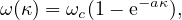
the law governing the evolution of the damage variable
| (242) |
and the hardening law
| (243) |
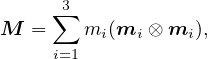
In the equations above, is the effective stress tensor, D is the elastic stiffness tensor, f is the yield function, λ is the consistency parameter (plastic multiplier), ω is the damage variable, σY is the yield stress and s, a, σH and ωc are positive material parameters. Material anisotropy is characterized by the second-order positive definite fabric tensor
| (244) |
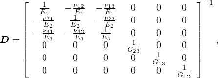
normalized such that Tr(M) = 3, mi are the eigenvalues and mi the eigenvectors. The eigenvectors of the fabric tensor determine the directions of material orthotropy and the components of the elastic stiffness tensor D are linked to eigenvalues of the fabric tensor. In the coordinate system aligned with mi, i = 1,2,3, the stiffness can be presented in Voigt (engineering) notation as
| (245) |
where Ei = E0ρkmi2l, Gij = G0ρkmilmjl and νij = ν0 . Here, E0, G0 and ν0 are elastic constants characterizing
the compact (poreless) material, ρ is the volume fraction of solid phase and k and l are dimensionless
exponents.
. Here, E0, G0 and ν0 are elastic constants characterizing
the compact (poreless) material, ρ is the volume fraction of solid phase and k and l are dimensionless
exponents.
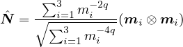
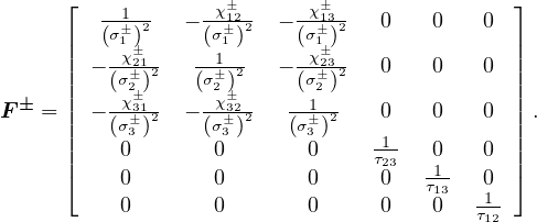
Similar relations as for the stiffness tensor are also postulated for the components of a fourth-order tensor F that
is used in the yield condition. The yield condition is divided into tensile and compressive parts. Tensor F is different
in each part of the effective stress space. This tensor is denoted F+ in tensile part, characterized by  : ≤ 0 and
F- in compressive part, characterized by
: ≤ 0 and
F- in compressive part, characterized by  : ≤ 0, where
| (246) |
| (247) |
In the equation above σi± = σ0±ρpmi2q is uniaxial yield stress along the i-th principal axis of orthotropy,
τij = τ0ρpmiqmjq is the shear yield stress in the plane of orthotropy and χij± = χ0± is the so-called interaction
coefficient, p and q are dimensionless exponents and parameters with subscript 0 are related to a fictitious material
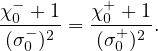
with zero porosity. The yield surface is continuously differentiable if the parameters values are constrained by the
condition
is the so-called interaction
coefficient, p and q are dimensionless exponents and parameters with subscript 0 are related to a fictitious material
with zero porosity. The yield surface is continuously differentiable if the parameters values are constrained by the
condition
| (248) |
The model description and parameters are summarized in Tab. 51.
| Description | Anisotropic elastoplastic model with isotropic damage |
| Record Format | TrabBone3d (in) # d(rn) # eps0(rn) # nu0(rn) # mu0(rn) # expk(rn) # expl(rn) # m1(rn) # m2(rn) # rho(rn) # sig0pos(rn) # sig0neg(rn) # chi0pos(rn) # chi0neg(rn) # tau0(rn) # plashardfactor(rn) # expplashard(rn) # expdam(rn) # critdam(rn) # |
| Parameters | - material number |
| - d material density |
|
| - eps0 Young modulus (at zero porosity) |
|
| - nu0 Poisson ratio (at zero porosity) |
|
| - mu0 shear modulus of elasticity (at zero porosity) |
|
| - m1 first eigenvalue of the fabric tensor |
|
| - m2 second eigenvalue of the fabric tensor |
|
| - rho volume fraction of solid phase |
|
| - sig0pos yield stress in tension |
|
| - sig0neg yield stress in compression |
|
| - tau0 yield stress in shear |
|
| - chi0pos interaction coefficient in tension |
|
| - plashardfactor hardening parameter |
|
| - expplashard exponent in hardening law |
|
| - expdam exponent in damage law |
|
| - critdam critical damage |
|
| - expk exponent k in the expression for elastic stiffness |
|
| - expl exponent l in the expression for elastic stiffness |
|
| - expq exponent q in the expression for tensor F |
|
| - expp exponent p in the expression for tensor F |
|
| Supported modes | 3dMat |
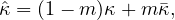
The model is regularized by the over-nonlocal formulation with damage driven by a combination of local and nonlocal cumulated plastic strain
| (249) |
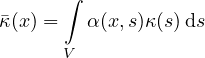
where m is a dimensionless material parameter (typically m > 1) and
| (250) |
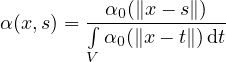
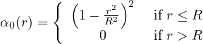
is the nonlocal cumulated plastic strain. The nonlocal weight function is defined as
| (251) |
where
| (252) |
Parameter R is related to the internal length of the material. The model description and parameters are summarized in Tab. 52.
| Description | Nonlocal anisotropic elastoplastic model with isotropic damage |
| Record Format | TrabBoneNL3d (in) # d(rn) # eps0(rn) # nu0(rn) # mu0(rn) # expk(rn) # expl(rn) # m1(rn) # m2(rn) # rho(rn) # sig0pos(rn) # sig0neg(rn) # chi0pos(rn) # chi0neg(rn) # tau0(rn) # plashardfactor(rn) # expplashard(rn) # expdam(rn) # critdam(rn) # m(rn) # R(rn) # |
| Parameters | - material number |
| - d material density |
|
| - eps0 Young modulus (at zero porosity) |
|
| - nu0 Poisson ratio (at zero porosity) |
|
| - mu0 shear modulus (at zero porosity) |
|
| - m1 first eigenvalue of the fabric tensor |
|
| - m2 second eigenvalue of the fabric tensor |
|
| - rho volume fraction of the solid phase |
|
| - sig0pos yield stress in tension |
|
| - tau0 yield stress in shear |
|
| - chi0pos interaction coefficient in tension |
|
| - chi0neg interaction coefficient in compression |
|
| - plashardfactor hardening parameter |
|
| - expplashard exponent in the hardening law |
|
| - expdam exponent in the damage law |
|
| - critdam critical damage |
|
| - expk exponent k in the expression for elastic stiffness |
|
| - expl exponent l in the expression for elastic stiffness |
|
| - expq exponent q in the expression for tensor F |
|
| - expp exponent p in the expression for tensor F |
|
| - m over-nonlocal parameter |
|
| - R nonlocal interaction radius |
|
| Supported modes | 3dMat |