This isotropic damage model assumes that the stiffness degradation is isotropic, i.e., stiffness moduli corresponding to different directions decrease proportionally and independently of direction of loading. It introduces two damage parameters ωt and ωc that are computed from the same equivalent strain using two different damage functions gt and gc. The gt is identified from the uniaxial tension tests, while gc from compressive test. The damage parameter for general stress states ω is obtained as a linear combination of ωt and ωc: ω = αtgt + αcgc, where the coefficients αt and αc take into account the character of the stress state. The damaged stiffness tensor is expressed as D = (1 - ω)De. Damage evolution law is postulated in an explicit form, relating damage parameter and scalar measure of largest reached strain level in material, taking into account the principle of preserving of fracture energy Gf. The equivalent strain, i.e., a scalar measure of the strain level is defined as norm from positive principal strains. The model description and parameters are summarized in Tab. 33.
| Description | Mazars damage model for concrete |
| Record Format | MazarsModel d(rn) # E(rn) # n(rn) # e0(rn) # ac(rn) # [bc(rn) #] [beta(rn) #] at(rn) # [ bt(rn) #] [hreft(rn) #] [hrefc(rn) #] [version(in) #] [tAlpha(rn) #] [equivstraintype(in) #] [maxOmega(rn) #] |
| Parameters | - num material model number |
| - d material density | |
| - E Young modulus | |
| - n Poisson ratio |
|
| - e0 max effective strain at peak |
|
| - ac,bc material parameters related to the shape of uniaxial compression curve (A sample set used by Saouridis is Ac = 1.34,Bc = 2537 |
|
| - beta coefficient reducing the effect of damage under response under shear. Default value set to 1.06 |
|
| - at, [bt] material parameters related to the shape of uniaxial tension curve. Meaning dependent on version parameter. |
|
| - hreft, hrefc reference characteristic lengths for tension and compression. The material parameters are specified for element with these characteristic lengths. The current element then will have the same COD (Crack Opening Displacement) as reference one. |
|
| - version Model variant. if 0 specified, the original form gt = 1.0 - (1.0 - At) * ε0∕κ - At * exp(-Bt * (κ - ε0)); of tension damage evolution law is used, if equal 1, the modified law used which asymptotically tends to zero gt = 1.0 - (ε0∕κ) * exp((ε0 - κ)∕εf) |
|
| - tAlpha thermal dilatation coefficient |
|
| - equivstraintype see Tab. 26 |
|
| - maxOmega limit maximum damage, use for convergency improvement |
|
| Supported modes | 3dMat, PlaneStress, PlaneStrain, 1dMat |
The nonlocal variant of Mazars damage model for concrete. Model based on nonlocal averaging of equivalent strain. The nonlocal averaging acts as a powerful localization limiter. The bell-shaped nonlocal averaging function is used. The model description and parameters are summarized in Tab. 34.
| Description | Nonlocal Mazars damage model for concrete |
| Record Format | MazarsModelnl r(rn) # E(rn) # n(rn) # e0(rn) # ac(rn) # bc(rn) # beta(rn) # version(in) # at(rn) # [ bt(rn) #] r(rn) # tAlpha(rn) # |
| Parameters | - num material model number |
| - d material density | |
| - E Young modulus | |
| - n Poisson ratio |
|
| - maxOmega limit maximum damage, use for convergency improvement |
|
| - tAlpha thermal dilatation coefficient |
|
| - version Model variant. if 0 specified, the original form gt = 1.0 - (1.0 - At) * ε0∕κ - At * exp(-Bt * (κ - ε0)); of tension damage evolution law is used, if equal 1, the modified law used which asymptotically tends to zero gt = 1.0 - (ε0∕κ) * exp((ε0 - κ)∕At) |
|
| - ac,bc material parameters related to the shape of uniaxial compression curve (A sample set used by Saouridis is Ac = 1.34,Bc = 2537 |
|
| - at, [bt] material parameters related to the shape of uniaxial tension curve. Meaning dependent on version parameter. |
|
| - beta coefficient reducing the effect of damage under response under shear. Default value set to 1.06 |
|
| - r parameter specifying the width of nonlocal averaging zone |
|
| Supported modes | 3dMat, PlaneStress, PlaneStrain, 1dMat |
Implementation of aging viscoelastic model for concrete creep according to the CEB-FIP Model Code. The model parameters are summarized in Tab. 35.
| Description | CebFip78 model for concrete creep with aging |
| Record Format | CebFip78 n(rn) # relMatAge(rn) # E28(rn) # fibf(rn) # kap_a(rn) # kap_c(rn) # kap_tt(rn) # u(rn) # |
| Parameters | - num material model number |
| - E28 Young modulus at age of 28 days [MPa] |
|
| - n Poisson ratio | |
| - fibf basic creep coefficient | |
| - kap_a coefficient of hydrometric conditions |
|
| - kap_c coefficient of type of cement |
|
| - kap_tt coeficient of temperature effects |
|
| - u surface imposed to environment [mm2]; temporary here; should be in crosssection level |
|
| - relmatage relative material age |
|
| Supported modes | 3dMat, PlaneStress, PlaneStrain, 1dMat, 2dPlateLayer,2dBeamLayer, 3dShellLayer |
Implementation of aging viscoelastic model for concrete creep with compliance function given by the double-power law. The model parameters are summarized in Tab. 36.
| Description | Double-power law model for concrete creep with aging |
| Record Format | DoublePowerLaw n(rn) # relMatAge(rn) # E28(rn) # fi1(rn) # m(rn) # n(rn) # alpha(rn) # |
| Parameters | - num material model number |
| - E28 Young modulus at age of 28 days [MPa] |
|
| - n Poisson ratio | |
| - fibf basic creep coefficient |
|
| - m coefficient |
|
| - n coefficient |
|
| - alpha coeficient |
|
| - relmatage relative material age |
|
| Supported modes | 3dMat, PlaneStress, PlaneStrain, 1dMat, 2dPlateLayer,2dBeamLayer, 3dShellLayer |
Implementation of aging viscoelastic model for concrete creep according to Eurocode 2 for concrete structures The model parameters are summarized in Tab. 37.
According to EC2, the compliance function is defined using the creep coefficient φ as
where Ecm is the mean elastic modulus at the age of 28 days and E(t′) is the elastic modulus at the age of loading, t′.
Current implementation supports only linear creep which is valid only for stresses below 0.45 of the characteristic compressive strength at the time of loading.
The elastic modulus at age t (in days) is defined as
![[ ( ( ∘ ---))]0.3
E(t) = exp s 1 - 28∕t Ecm (97)](matlibmanual159x.png)
where s is a cement-type dependent constant (0.2 for class R, 0.25 for class N and finally 0.38 for type S), and the mean secant elastic modulus at 28 days can be estimated from the mean compressive strength

where fcm,28 is in MPa and the resulting modulus is in GPa.
The creep coefficient is given by the expression from Annex B of the standard.

with
and

else
and t′T is the temperature-adusted age according to B.9 in the code. It is computed automatically if string temperatureDependent appears in the input record.
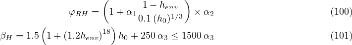
The shrinkage deformation is additively split into two parts: drying shrinkage εsh,d and autogenous shrinkage εsh,a. Drying shrinkage strain at time t is computed from

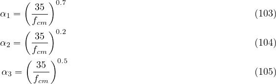
where t0 is the duration of curing, kh is a thickness-dependent parameter and
 (107)
env](matlibmanual166x.png)
with αds1 = 3 for cement class S, 4 for class N, and 6 for class R, and αds2 = 0.13 for cement class S, 0.12 for class N, and 0.11 for class R.
Autogenous shrinkage strain can be comptued as
![[ ( √-)] -6
εsh,a = 2.5(fcm - 18) 1- exp - 0.2 t × 10 (108)](matlibmanual167x.png)
| Description | EC2CreepMat model for concrete creep and shrinkage |
| Record Format | EC2CreepMat n(rn) # [ begOfTimeOfInterest(rn) #] [ endOfTimeOfInterest(rn) #] relMatAge(rn) # [ timeFactor(rn) #] stiffnessFactor(rn) # [ tAlpha(rn) #] fcm28(rn) # t0(rn) # cemType(in) # [ henv(rn) #] h0(rn) # shType(in) # [ spectrum ] [ temperatureDependent ] |
| Parameters | - num material model number |
| - n Poisson’s ratio |
|
| - begOfTimeOfInterest determines the shortest time which is reasonably well captured by the approximated compliance function (default value is 0.1); the units are the time units of the analysis |
|
| - endOfTimeOfInterest determines the longest time which is reasonably well captured by the approximated compliance function (if not provided it is read from the engineering model); the units are the time units of the analysis |
|
| - relMatAge time shift used to specify the age of material on the begging of the analysis, the meaning is the material age at time t = 0; |
|
| - timeFactor scaling factor transforming the actual time into appropriate units needed by the formulae of the eurocode. For analysis in days timeFactor = 1, for analysis in seconds timeFactor = 86,400. |
|
| - stiffnessFactor scaling factor transforming predicted stiffness into appropriate units of the analysis, for analysis in MPa stiffnessFactor = 1.e6 (default), for Pa stiffnessFactor = 1 |
|
| - fcm28 mean compressive strength measured on cylinders at the age of 28 days in MPa |
|
| - t0 duration of curing [day] (this is relevant only for drying shrinkage, not for creep) |
|
| - cemType type of cement, 1 = class R, 2 = class N, 3 = class S |
|
| - henv ambient relative humidity expressed as decimal |
|
| - h0 effective member thickness in [mm] calculated according to EC2 as 2×A/u where A is the cross-section are and u is the cross-section perimeter exposed to drying |
|
| - shType shrinkage type; 0 = no shrinkage, 1 = both drying and autogenous shrinkage, 2 = drying shrinkage only, 3 = autogenous shrinkage only |
|
| - spectrum this string switches on evaluation of the moduli of the aging Kelvin chain using the retardation spectrum of the compliance function, otherwise (default option) the least-squares method is used |
|
| - temperatureDependent turns on the influence of temperature on concrete maturity (equivalent age concept) by default this option is not activated. |
|
| Supported modes | 3dMat, PlaneStress, PlaneStrain, 1dMat, 2dPlateLayer,2dBeamLayer, 3dShellLayer |
Model B3 is an aging viscoelastic model for concrete creep and shrinkage, developed by Prof. Bažant and coworkers. In OOFEM it is implemented in three different ways.
The first version, “B3mat”, is kept in OOFEM for compatibility. It is based on an aging Maxwell chain. The moduli of individual units in the chain are evaluated in each step using the least-squares method.
The second, more recent version, is referred to as “B3solidmat”. Depending on the specified input it exploits either a non-aging Kelvin chain combined with the solidification theory, or an aging Kelvin chain. It is extended to the so-called Microprestress-Solidification theory (MPS), which in this implementation takes into account only the effects of variable humidity on creep; the effects of temperature on creep are not considered. The underlying rheological chain consists of four serially coupled components. The solidifying Kelvin chain represents short-term creep; it is serially coupled with a non-aging elastic spring that reflects instantaneous deformation. Long-term creep is captured by an aging dashpot with viscosity dependent on the microprestress, the evolution of which is affected by changes of humidity. The last unit describes volumetric deformations (shrinkage and thermal strains). Drying creep is incorporated either by the “averaged cross-sectional approach”, or by the “point approach”.
The latest version is denoted as “MPS” and is based on the microprestress-solidification theory [29] [30] [31]. The rheological model consists of the same four components as in “B3solidmat”, but now the implemented exponential algorithm is designed especially for the solidifying Kelvin chain, which is a special case of an aging Kelvin chain. This model takes into account both humidity and temperature effects on creep. Drying creep is incorporated exclusively by the so-called “point approach”. The model can operate in four modes, controlled by the keyword CoupledAnalysisType. The first mode (CoupledAnalysisType = 0) solves only the basic creep and runs as a single problem, while the remaining three modes need to be run as a staggered problem with humidity and/or temperature analysis preceding the mechanical problem; both humidity and temperature fields are read when CoupledAnalysisType = 1, only the field of relative humidity is taken into account when CoupledAnalysisType = 2 and finally, only temperature when CoupledAnalysisType = 3.
The basic creep is in the microprestress-solidification theory influenced by the same four parameters q1 - q4 as in the model B3. Values of these parameters can be estimated from the composition of concrete mixture and its compressive strength using the following empirical formulae:
![- 0.5
q1 = 126.77¯fc [10-6∕MPa ] (109)
q2 = 185.4c0.5¯fc- 0.9 [10-6∕MPa ] (110)
4 -6
q3 = 0.29(w∕c) q2 [10 ∕MPa ] (111)
q4 = 20.3(a∕c)- 0.7 [10-6∕MPa ] (112)](matlibmanual168x.png)
Here, is the average compressive cylinder strength at age of 28 days [MPa], a, w and c is the weight of aggregates, water and cement per unit volume of concrete [kg/m3].
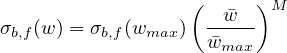
The non-aging spring stiffness represents the asymptotic modulus of the material; it is equal to 1∕q1. The
solidifying Kelvin chain is composed of M Kelvin units with fixed retardation times τμ, μ = 1,2,…,M, which form a
geometric progression with quotient 10. The lowest retardation time τ1 is equal to 0.3 begoftimeofinterest, the
highest retardation time τM is bigger than 0.5 endoftimeofinterest. The chain also contains a spring with stiffness
E0∞ (a special case of Kelvin unit with zero retardation time). Moduli Eμ∞ of individual Kelvin units
are determined such that the chain provides a good approximation of the non-aging micro-compliance
function of the solidifying constituent, Φ(t - t′) = q2 ln , where λ
0 = 1 day and
n = 0.1. The technique based on the continuous retardation spectrum leads to the following formulae:
, where λ
0 = 1 day and
n = 0.1. The technique based on the continuous retardation spectrum leads to the following formulae:
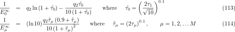
Viscosities ημ∞ of individual Kelvin units are obtained from simple relation ημ∞ = τμ∕Eμ∞. A higher accuracy is reached if all retardation times are in the end multiplied by the factor 1.35 and the last modulus EM is divided by 1.2.
The actual viscosities ημ and stiffnesses Eμ of the solidifying chain change in time according to ημ(t) = v(t)ημ∞ and Eμ(t) = v(t)Eμ∞, where
| (115) |
is the volume growth function, and exponent m = 0.5. In the case of variable temperature or humidity, the actual age of concrete t is replaced by the equivalent time te, which is obtained by integrating (118).
Evolution of viscosity of the aging dashpot is governed by the differential equation
| (116) |
where h is the relative pore humidity, T is the absolute temperature [K], T0 = 298 K is the room temperature, and parameter p = 2. Parameter kT is different for monotonically increasing and for cyclic temperature, and is defined as
| (117) |
in which kTm [-] and kTc [-] are new parameters and Tmax is the maximum temperature attained in the previous history of the material point.
Equation (116) differs from the one presented in the original work; it replaces the differential equation for microprestress, which is not used here. The evolution of viscosity can be captured directly, without the need for microprestress. What matters is only the relative humidity and temperature and their rates. Parameters c0 and k1 of the original MPS theory are replaced by μS = c0T0p-1k1p-1q4(p - 1)p. The initial value of viscosity is defined as η(t0) = t0∕q4, where t0 is age of concrete at the onset drying or when the temperature starts changing, in the present implementation it is set relMatAge which corresponds to the material age when the material is cast.
As mentioned above, under variable humidity and temperature conditions the physical time t in function v(t) describing evolution of the solidified volume is replaced by the equivalent time te. In a similar spirit, t is replaced by the solidification time ts in the equation describing creep of the solidifying constituent, and by the reduced time tr in equation dεf∕dtr = σ∕η(t) relating the flow strain rate to the stress. Factors transforming the physical time t into te, tr and ts are defined as follows:
Functions describing the influence of temperature have the form
![[ ( ) ]
β (T ) = exp Qe- 1-- 1- (121)
eT R T0 T
[Qr ( 1 1) ]
βrT(T ) = exp -R- T-- T- (122)
[ ( 0 ) ]
βsT(T ) = exp Qs- 1-- 1- (123)
R T0 T](matlibmanual175x.png)
motivated by the rate process theory. R is the universal gas constant and Qe, Qr, Qs are activation energies for hydration, viscous processes and microprestress relaxation, respectively. Only the ratios Qe∕R, Qr∕R and Qs∕R have to be specified. Functions describing the influence of humidity have the form
![1
βeh(h) = ------------4- (124)
1+ [αe(1- h)]2
βrh(h) = αr + (1- αr)h (125)
βsh(h) = αs + (1- αs)h2 (126)](matlibmanual176x.png)
where αe, αr and αs are parameters.
At sealed conditions (or CoupledAnalysisType = 2) the auxiliary coefficients βeT = βrT = βsT = 1 while at room temperature (or with CoupledAnalysisType = 3) factors βe,h = βr,h = βs,h = 1.
It turned out that both the size effect on drying creep as well as its delay behind drying shrinkage can be addressed through parameter p in the governing equation (116). In the experiments, the average (cross-sectional) drying creep is decreasing with specimen size. Unfortunately, for the standard value p = 2, the MPS model exhibits the opposite trend. For p = ∞ the size effect disappears, and for p < 0 it corresponds to the experiments. It should be noted that for negative or infinite values of p the underlying theory loses its original physical background. If the experimental data of drying creep measured on different sizes are missing, the exponent p = ∞ can be taken as a realistic estimate.
When parameter p is changed from its recommended value p = 2 it is advantageous to rewrite the governing differential equation to the following form
| (127) |
with newly introduced parameters
| (128) |
| (129) |
With the “standard value” p = 2 (reverted size effect) the new parameter  is also 2, for p < 0 (correct size effect)
 < 1 and finally with p = ∞ the first parameter
  = 1 and the second parameter k3 becomes dimensionless. The
other advantage of
= 1 and the second parameter k3 becomes dimensionless. The
other advantage of  = 1 is that the governing differential equation becomes linear and can be solved
directly.
= 1 is that the governing differential equation becomes linear and can be solved
directly.
The rate of thermal strain is expressed as  T = αTṪ and the rate of drying shrinkage strain as
  sh = kshḣ, where
both αT and ksh are assumed to be constant in time and independent of temperature and humidity.
sh = kshḣ, where
both αT and ksh are assumed to be constant in time and independent of temperature and humidity.
There are two options to simulate the autogenous shrinkage in the MPS material model. The first one is according to the B4 model
| (130) |
and the second one is proposed in the Model Code 2010
| (131) |
For the normally hardening cement, the ultimate value of the autogenous shrinkage can be estimated from the composition using the empirical formula of the B4 model
Similarly, in the Model Code, the ultimate shrinkage strain can be estimated from the mean concrete strength at the age of 28 days and from the cement grade
where αas is 600 for cement grades 42.5 R and 52.5 R and N, 700 for 32.5 R and 42.5 N and 800 for 32.5 N.
The model description and parameters are summarized in Tab. 38 for “B3mat”, in Tab. 39 for “B3solidmat”, and in Tab. 40 for “MPS”. Since some model parameters are determined from the composition and strength using empirical formulae, it is necessary to use the specified units (e.g. compressive strength always in MPa, irrespectively of the units used in the simulation for stress). For “B3mat” and “B3solidmat” it is strictly required to use the specified units in the material input record (stress always in MPa, time in days etc.). The “MPS” model is almost unit-independent, except for c in MPa and c in kg/m3, which are used in empirical formulae.
| Description | B3 material model for concrete aging |
| Record Format | B3mat d(rn) # n(rn) # talpha(rn) # [ begoftimeofinterest(rn) #] [ endoftimeofinterest(rn) #] timefactor(rn) # relMatAge(rn) # [ mode(in) #] fc(rn) # cc(rn) # w/c(rn) # a/c(rn) # t0(rn) # q1(rn) # q2(rn) # q3(rn) # q4(rn) # shmode(in) # ks(rn) # vs(rn) # hum(rn) # [ alpha1(rn) #] [ alpha2(rn) #] kt(rn) # EpsSinf(rn) # q5(rn) # es0(rn) # r(rn) # rprime(rn) # at(rn) # w_h(rn) # ncoeff(rn) # a(rn) # |
| Parameters | - num material model number |
| - d material density | |
| - n Poisson ratio |
|
| - talpha coefficient of thermal expansion |
|
| - begoftimeofinterest optional parameter; lower boundary of time interval with good approximation of the compliance function [day]; default 0.1 day |
|
| - endoftimeofinterest optional parameter; upper boundary of time interval with good approximation of the compliance function [day] |
|
| - timefactor scaling factor transforming the simulation time units into days |
|
| - relMatAge relative material age [day] |
|
| - mode if mode = 0 (default value) creep and shrinkage parameters are predicted from composition; for mode = 1 parameters must be user-specified. |
|
| - fc 28-day mean cylinder compression strength [MPa] |
|
| - cc cement content of concrete [kg/m3] |
|
| - w/c ratio (by weight) of water to cementitious material |
|
| - a/c ratio (by weight) of aggregate to cement |
|
| - t0 age when drying begins [day] |
|
| - q1-q4 parameters of B3 model for basic creep [1/TPa] |
|
| - shmode shrinkage mode; 0 = no shrinkage; 1 = average shrinkage (the following parameters must be specified: ks, vs, hum and additionally alpha1 alpha2 for mode = 0 and kt EpsSinf q5 t0 for mode = 1; 2 = point shrinkage (needed: es0, r, rprime, at, w_h, ncoeff, a) |
|
| - ks cross-section shape factor [-] |
|
| - vs volume to surface ratio [m] |
|
| - hum relative humidity of the environment [-] |
|
| - alpha1 shrinkage parameter – influence of cement type [-] |
|
| - alpha2 shrinkage parameter – influence of curing type [-] |
|
| - kt shrinkage parameter [day/m2] |
|
| - EpsSinf shrinkage parameter [10-6] |
|
| - q5 drying creep parameter [1/TPa] |
|
| - es0 final shrinkage at material point |
|
| - r, rprime coefficients |
|
| - at oefficient relating stress-induced thermal strain and shrinkage |
|
| - w_h, ncoeff, a sorption isotherm parameters obtained from experiments [Pedersen, 1990] |
|
| Supported modes | 3dMat, PlaneStress, PlaneStrain, 1dMat, 2dPlateLayer,2dBeamLayer, 3dShellLayer |
For illustration, sample input records for the material considered in Example 3.1 of the creep book by Bažant and Jirásek is presented. The concrete mix is composed of 170 kg/m3 of water, 450 kg/m3 of type-I cement and 1800 kg/m3 of aggregates, which corresponds to ratios w∕c = 0.3778 and a∕c = 4. The compressive strength is c = 45.4 MPa. The concrete slab of thickness 200 mm is cured in air with initial protection against drying until the age of 7 days. Subsequently, the slab is exposed to an environment with relative humidity of 70%. The following input record can be used for the first version of the model (B3mat):
B3mat 1 n 0.2 d 0. talpha 1.2e-5 relMatAge 28. fc 45.4 cc 450. w/c 0.3778 a/c 4. t0 7. timefactor 1. alpha1 1. alpha2 1.2 ks 1. hum 0.7 vs 0.1 shmode 1
Parameter α1 = 1 corresponds to type-I cement, parameter α2 = 1.2 to curing in air, parameter ks = 1 to an infinite slab. The volume-to-surface ratio is in this case equal to one half of the slab thickness and must be specified in meters, independently of the length units that are used in the finite element analysis (e.g., for nodal coordinates). The value of relMatAge must be specified in days. Parameter relMatAge 28. means that time 0 of the analysis corresponds to concrete age 28 days. If material B3mat is used, the finite element analysis must use days as the units of time (not only for relMatAge, but in general, e.g. for the time increments).
If only the basic creep (without shrinkage) should be computed, then the material input record reduces to following: B3mat 1 n 0.2 d 0. talpha 1.2e-5 relMatAge 28. fc 45.4 cc 450. w/c 0.3778 a/c 4. t0 7. timefactor 1. shmode 0
| Description | B3solid material model for concrete creep |
| Record Format | B3solidmat d(rn) # n(rn) # talpha(rn) # mode(in) # [ EmoduliMode(in) #] Microprestress(in) # shm(in) # [ begoftimeofinterest(rn) #] [ endoftimeofinterest(rn) #] timefactor(rn) # relMatAge(rn) # fc(rn) # cc(rn) # w/c(rn) # a/c(rn) # t0(rn) # q1(rn) # q2(rn) # q3(rn) # q4(rn) # c0(rn) # c1(rn) # tS0(rn) # w_h(rn) # ncoeff(rn) # a(rn) # ks(rn) # [ alpha1(rn) #] [ alpha2(rn) #] hum(rn) # vs(rn) # q5(rn) # kt(rn) # EpsSinf(rn) # es0(rn) # r(rn) # rprime(rn) # at(rn) # kSh(rn) # inithum(rn) # finalhum(rn) # |
| Parameters | - num material model number |
| - d material density | |
| - n Poisson ratio |
|
| - talpha coefficient of thermal expansion |
|
| - mode optional parameter; if mode = 0 (default), parameters q1 - q4 are predicted from composition of the concrete mixture (parameters fc, cc, w/c, a/c and t0 need to be specified). Otherwise values of parameters q1-q4 are expected. |
|
| - EmoduliMode optional parameter; analysis of retardation spectrum (= 0, default value) or least-squares method (= 1) is used for evaluation of Kelvin units moduli |
|
| - Microprestress 0 = basic creep; 1 = drying creep (must be run as a staggered problem with preceding analysis of humidity diffusion. Parameter shm must be equal to 3. The following parameters must be specified: c0, c1, tS0, w_h, ncoeff, a) |
|
| - shmode shrinkage mode; 0 = no shrinkage; 1 = average shrinkage (the following parameters must be specified: ks, vs, hum and additionally alpha1 alpha2 for mode = 0 and kt EpsSinf q5 for mode = 1; 2 = point shrinkage (needed: es0, r, rprime, at), w_h ncoeff a; 3 = point shrinkage based on MPS theory (needed: parameter kSh or value of kSh can be approximately determined if following parameters are given: inithum, finalhum, alpha1 and alpha2) |
|
| - begoftimeofinterest optional parameter; lower boundary of time interval with good approximation of the compliance function [day]; default 0.1 day |
|
| - endoftimeofinterest optional parameter; upper boundary of time interval with good approximation of the compliance function [day] |
|
| - timefactor scaling factor transforming the simulation time units into days |
|
| - relMatAge relative material age [day] |
|
| - fc 28-day mean cylinder compression strength [MPa] |
|
| - cc cement content of concrete mixture [kg/m3] |
|
| - w/c water to cement ratio (by weight) |
|
| - a/c aggregate to cement ratio (by weight) |
|
| - t0 age of concrete when drying begins [day] |
|
| - q1, q2, q3, q4 parameters (compliances) of B3 model for basic creep [1/TPa] |
|
| - c0 MPS theory parameter [MPa-1 day-1] |
|
| - c1 MPS theory parameter [MPa] |
|
| - tS0 MPS theory parameter - time when drying begins [day] |
|
| - w_h, ncoeff, a sorption isotherm parameters obtained from experiments [Pedersen, 1990] |
|
| - ks cross section shape factor [-] |
|
| - alpha1 optional shrinkage parameter - influence of cement type (optional parameter, default value is 1.0) |
|
| - alpha2 optional shrinkage parameter - influence of curing type (optional parameter, default value is 1.0) |
|
| - hum relative humidity of the environment [-] |
|
| - vs volume to surface ratio [m] |
|
| - q5 drying creep parameter [1/TPa] |
|
| - kt shrinkage parameter [day/m2] |
|
| - EpsSinf shrinkage parameter [10-6] |
|
| - es0 final shrinkage at material point |
|
| - at coefficient relating stress-induced thermal strain and shrinkage |
|
| - rprime, r coefficients |
|
| - kSh influences magnitude of shrinkage in MPS theory [-] |
|
| - inithum [-], finalhum [-] if provided, approximate value of kSh can be computed |
|
| Supported modes | 3dMat, PlaneStress, PlaneStrain, 1dMat, 2dPlateLayer, 2dBeamLayer, 3dShellLayer |
Now consider the same conditions for “B3solidmat”. In all the examples below, the input record with the material
description can start by
B3solidmat 1 d 2420. n 0.2 talpha 12.e-6 begtimeofinterest 1.e-2
endtimeofinterest 3.e4 timefactor 86400. relMatAge 28.
Parameters begoftimeofinterest 1.e-2 and endoftimeofinterest 3.e4 mean that the computed response (e.g., deflection) should be accurate in the range from 0.01 day to 30,000 days after load application. Parameter timefactor 86400. means that the time unit used in the finite element analysis is 1 second (because 1 day = 86,400 seconds). Note that the values of begtimeofinterest, endtimeofinterest and relMatAge are always specified in days, independently of the actual time units in the analysis. Parameter EmoduliMode is not specified, which means that the moduli of the Kelvin chain will be determined using the default method, based on the continuous retardation spectrum.
Additional parameters depend on the specific type of analysis:
Computing basic creep only, shrinkage not considered, parameters qi estimated from composition.
mode 0 fc 45.4 cc 450. w/c 0.3778 a/c 4.
t0 7. microprestress 0 shmode 0
Computing basic creep only, shrinkage not considered, parameters qi specified by the user.
mode 1 q1 18.81 q2 126.9 q3 0.7494 q4 7.692
microprestress 0 shmode 0
Computing basic creep only, shrinkage handled using the sectional approach, parameters estimated from
composition.
mode 0 fc 45.4 cc 450. w/c 0.3778 a/c 4. t0 7.
microprestress 0 shmode 1 ks 1. alpha1 1. alpha2 1.2 hum 0.7 vs 0.1
Computing basic creep only, shrinkage handled using the sectional approach, parameters specified by the
user.
mode 1 q1 18.81 q2 126.9 q3 0.7494 q4 7.692
microprestress 0 shmode 1 ks 1. q5 326.7 kt 28025 EpsSinf 702.4 t0 7. hum 0.7 vs 0.1
Computing basic creep only, shrinkage handled using the point approach (B3), parameters specified by
the user.
mode 1 q1 18.81 q2 126.9 q3 0.7494 q4 7.692
microprestress 0 shmode 2 es0 ... r ... rprime ... at ...
Computing drying creep, shrinkage handled using the point approach (MPS), parameters qi estimated
from composition.
mode 0 fc 45.4 w/c 0.3778 a/c 4. t0 7. microprestress 1
shmode 3 c0 1. c1 0.2 tS0 7. w_h 0.0476 ncoeff 0.182 a 4.867 kSh 1.27258e-003
| Description | Microprestress-solidification theory material model for concrete creep |
| Record Format | mps d(rn) # n(rn) # talpha(rn) # referencetemperature(rn) # mode(in) # [ CoupledAnalysisType(in) #] [ begoftimeofinterest(rn) #] [ endoftimeofinterest(rn) #] timefactor(rn) # relMatAge(rn) # lambda0(rn) # fc(rn) # cc(rn) # w/c(rn) # a/c(rn) # stiffnessfactor(rn) # q1(rn) # q2(rn) # q3(rn) # q4(rn) # ksh(rn) # [ mus(rn) #] k3(rn) # [ alphaE(rn) #] [ alphaR(rn) #] [ alphaS(rn) #] [ QEtoR(rn) #] [ QRtoR(rn) #] [ QStoR(rn) #] kTm(rn) # [ kTc(rn) #] [ p(rn) #] [ p_tilde(rn) #] [ alpha_as(rn) #] [ eps_cas0(rn) #] [ b4_eps_au_infty(rn) #] [ b4_tau_au(rn) #] [ b4_alpha(rn) #] [ b4_r_t(rn) #] [ b4_cem_type(rn) #] [ temperInCelsius ] |
| Parameters | - num material model number |
| - d material density | |
| - n Poisson ratio |
|
| - talpha coefficient of thermal expansion |
|
| - referencetemperature reference temperature only to thermal expansion of material |
|
| - mode optional parameter; if mode = 0 (default), parameters q1 - q4 are predicted from composition of the concrete mixture (parameters fc, cc, w/c, a/c and stiffnessfactor need to be specified). Otherwise values of parameters q1 - q4 are expected. |
|
| - CoupledAnalysisType 0 = basic creep; 1 = (default) drying creep, shrinkage, temperature transient creep and creep at elevated temperature; 2 = drying creep, shrinkage; 3 = temperature transient creep and creep at elevated temperature; for choice # 1, 2, 3 the problem must be run as a staggered problem with preceding analysis of humidity and/or temperature distribution; Following parameters must be specified: mus or k3 (according to exponent p), kTm (compulsory for choice #3 otherwise optional) |
|
| - lambda0 scaling factor equal to 1.0 day in time units of analysis (e.g. 86400 if the analysis runs in seconds) |
|
| - begoftimeofinterest lower boundary of time interval with good approximation of the compliance function; default value = 0.01 lambda0 |
|
| - endoftimeofinterest upper boundary of time interval with good approximation of the compliance function; default value = 10000. lambda0 |
|
| - timefactor scaling factor, for mps material must be equal to 1.0 |
|
| - relMatAge relative material age = age at time when the material is cast in the structure |
|
| - fc 28-day standard cylinder compression strength [MPa] |
|
| - cc cement content of concrete mixture [kg m-3] |
|
| - w/c water to cement weight ratio |
|
| - a/c aggregate to cement weight ratio |
|
| - stiffnessfactor scaling factor converting “predicted” parameters q1 - q4 into proper units (e.g. 1.0 if stiffness is measured in Pa, 1.e6 for MPa) |
|
| - q1, q2, q3, q4 parameters of B3 model for basic creep |
|
| - p and p_tilde replaceable parameters in the governing equation for viscosity, default value is p = 2 |
|
| - mus parameter governing to the evolution of viscosity; for exponent p = 2, μS = c0c1q4 [Pa-1 s-1] |
|
| - k3 dimensionless parameter governing to the evolution of viscosity replacing mus in the special case when p > 100 (then p is automatically set to ∞ which is equivalent to p_tilde = 1) |
|
| - ksh parameter relating rate of shrinkage to rate of humidity [-], default value is 0.0, i.e. no shrinkage |
|
| - alphaE constant, default value 10. |
|
| - alphaR constant, default value 0.1 |
|
| - alphaS constant, default value 0.1 |
|
| - QEtoR activation energy ratio, default value 2700. K |
|
| - QRtoR activation energy ratio, default value 5000. K |
|
| - QStoR activation energy ratio, default value 3000. K |
|
| - kTm replaces lnh in the governing equation for viscosity |
|
| - kTc controls creep at cyclic temperature |
|
| - alpha_as and eps_cas0 control the ultimate value of autogenous shrinkage according to fib Model Code 2010; this ultimate value can be provided either directly via eps_cas0 (negative value for contraction) or using alpha_as, see equation (133) |
|
| - b4_eps_au_infty, b4_tau_au, b4_alpha, b4_r_t, b4_cem_type control the evolution and the ultimate value of autogenous shrinkage according to model B4; all parameters are predicted from composition if the b4_cem_type is provided; however, this prediction can be manually overridden |
|
| - temperInCelsius this string enables to run the supplementary transport problem with temperature in Celsius instead of Kelvin |
|
| Supported modes | 3dMat, PlaneStress, PlaneStrain, 1dMat, 2dPlateLayer, 2dBeamLayer, 3dShellLayer |
Finally consider the same conditions for “MPS material”. In all the examples below, the input record with the
material description can start by
mps 1 d 2420. n 0.2 talpha 12.e-6 referencetemperature 296.
Additional parameters depend on the specific type of analysis:
Computing basic creep only, shrinkage not considered, parameters qi estimated from composition and
simulation time in days and stiffnesses in MPa.
mode 0 fc 45.4 cc 450. w/c 0.3778 a/c 4. stiffnessFactor 1.e6
timefactor 1. lambda0 1. begoftimeofinterest 1.e-2
endoftimeofinterest 3.e4 relMatAge 28. CoupledAnalysisType 0.
Computing basic creep only, shrinkage not considered, parameters qi specified by user, simulation time
in seconds and stiffnesses in Pa.
mode 1 q1 18.81e-12 q2 126.9e-12 q3 0.7494e-12 q4 7.6926e-12
timefactor 1. lambda0 86400. begoftimeofinterest 864.
endoftimeofinterest 2.592e9 relMatAge 2419200. CoupledAnalysisType 0.
Computing both basic and drying creep, parameters qi specified by user, simulation time in seconds and
stiffnesses in MPa.
mode 1 q1 18.81e-6 q2 126.9e-6 q3 0.7494e-6 q4 7.6926e-6
timefactor 1. lambda0 86400. begoftimeofinterest 864.
endoftimeofinterest 2.592e9 relMatAge 2419200. CoupledAnalysisType 1.
ksh 0.0004921875. t0 2419200. kappaT 0.005051 mus 4.0509259e-8
Final recommendations:
to simulate basic creep without shrinkage it is possible to use all three models
B3mat with shmode = 0
B3Solidmat with shmode = 0 and microprestress = 0
MPS with CoupledAnalysisType = 0
to simulate drying creep with shrinkage using “sectional approach”, only the first material model (B3mat) is suitable can be used (with shmode = 1)
to simulate drying creep without shrinkage using “sectional approach”, only the first material model (B3mat) is suitable (with shmode = 1, mode = 1 and EpsSinf = 0.0)
to simulate drying creep with shrinkage using “point approach” according to B3 model there are two options:
B3mat (with shmode = 2)
B3Solidmat (with shmode = 2)
In order to suppress shrinkage set es0 = 0.0
to simulate drying creep with shrinkage using “point approach” according to MPS model there are two options:
B3Solidmat (with shmode = 3)
MPS with CoupledAnalysisType = 1
In order to suppress shrinkage set kSh = 0.0
This model extends the model based on the Microprestress-Solidification theory, described in previous section and summarized in Tab. 40 for “MPS”, by tensile cracking.
This extension uses the isotropic damage model with Rankine definition of the equivalent deformation defined as the biggest principal effective stress divided by the elastic modulus. The softening law cannot deal directly with the strain because due to creep strain increases and this would lead to further softening without additional loading.
Two different approaches are implemented. The first one, default, (#1) reduces the stiffness only in the directions of tension (in case the tensile strength is exceeded). A full stiffness is restored in compression and after unloading from tension.
The other approach (#2) is the standard isotropic damage model which reduces the stiffness equally in all directions independently of loading. This approach leads to faster convergence because the secant stiffness can be used instead of the incremental viscoelastic stiffness which must be used in the first approach. The second approach becomes useful when the loading is monotonic or when the benefit of the accelerated computation prevails over the consequences of the reduced/underestimated stiffness in compression.
Proper energy dissipation is guaranteed by the crack-band approach.
The following algorithm is used to compute the stress vector (in each time step and until the iteration criteria are met):
Compute effective stress
| (134) |
where σeff,k is the effective stress vector in the preceding step, k is the incremental stiffness, Dν is a unit stiffness matrix and Δεk, Δεk′′, Δεsh,k, ΔεT,k are the increments of the total strain, strain due to creep, shrinkage strain (sum of drying and autogenous shrinkage) and thermal strain, respectively.
Compute principal effective stresses σeff,1, σeff,2, σeff,3
Evaluate equivalent deformation
| (135) |
If the stress exceeds the material strength, initialize and fix the fracture parameters ft and GF (exponential softening assumed).
| (136) |
where h is the characteristic length of the finite element in the direction of the biggest principal stress.
Evaluate corresponding damage if  > ε0
> ε0
| (137) |
Compute principal nominal stresses
approach #1:
for i = 1,2,3
if σeff,i > 0, σi = (1 - ω)σeff,i
else σi = σeff,i
approach #2:
for i = 1,2,3
σi = (1 - ω)σeff,i
Construct the stress vector in the original configuration
| (138) |
where T is the stress transformation matrix.
The tensile strength and fracture energy can be defined either as fixed, time-independent values (parameters ft, gf) or as variable, depending on the equivalent hydration time te. The latter case is activated by keyword timeDepFracturing; tensile strength and fracture energy are then linked to the current value of the mean compressive strength using (slightly modified) formulae from the fib Model Code 2010.
For 0 MPa ≤ fcm(t) ≤ 20 MPa the tensile strength is computed from a linear function
| (139) |
which starts at the origin and at fcm(t) = 20 MPa connects to expression
| (140) |
which is valid for 20 MPa ≤ fcm(t) ≤ 58 MPa. Finally, for fcm(t) > 58 MPa
| (141) |
Following the guidelines from the Model Code 2010 (section 5.1.5.2), the fracture energy Gf can be estimated from the mean compressive strength at 28 days using an empirical formula
| (142) |
In this function, the mean compressive strength must be provided in MPa and the resulting fracture energy is in N/m.
The growth in fracture energy is approximately proportional to the tensile strength. The current value of fracture energy is very simply computed as
| (143) |
The development of the mean compressive strength in time is adopted entirely from the Model Code 2010 (see section 5.1.9.1)
| (144) |
where fib_s is a cement-type dependent coefficient (0.38 for cement 32.5 N; 0.25 for 32.5 R and 42.5 N; 0.2 for 42.5 R and 52.5 N and R), te is the equivalent age and fcm,28 is the mean compressive strength at the age of 28 days.
For some concretes the prediction formulae do not provide accurate predictions, therefore it is possible to scale the evolution of tensile strength and fracture energy by providing their 28-day values ft28 and gf28.
The model description and parameters are summarized in Tab. 41.
| Description | MPS damage model for concrete creep with cracking |
| (additionaly all parameters from Table 40) |
|
| Record Format | MPSDamMat [ ft(rn) #] [ gf(rn) #] [ timeDepFracturing ] [ fib_s(rn) #] [ ft28(rn) #] [ gf28(rn) #] [ damlaw(in) #] [ isotropic ] [ checksnapback(in) #] |
| Parameters | - ft tensile strength (constant in time) |
| - gf fracture energy (constant in time) |
|
| - timeDepFracturing string activating fib MC 2010 prediction for tensile strength and fracture energy + their time evolution |
|
| - ft28 manual override for the fib MC 2010 prediction of hydration-dependent tensile strength |
|
| - gf28 manual override for the fib MC 2010 prediction of hydration-dependent fracture energy |
|
| - fib_s cement-type dependent coefficient (compulsory with timeDepFracturing) |
|
| - damageLaw traction-separation law: 0 = exponential softening (default), 1 = linear softening, 6 = damage disabled |
|
| - isotropic string activating same reduction of stiffness after the onset of cracking both in in compression and tension (enables to use secant stiffness matrix for faster convergence) |
|
| - checkSnapBack switch for snap-back checking; 1 = activated (default), 0 = deactiavated |
|
| Supported modes | 3dMat, PlaneStress, PlaneStrain |
Model M4 covers inelastic behavior of concrete under complex triaxial stress states. It is based on the microplane concept and can describe softening. However, objectivity with respect to element size is not ensured – the parameters need to be manually adjusted to the element size. Since the tangent stiffness matrix is not available, elastic stiffness is used. This can lead to a very slow convergence when used within an implicit approach. The model parameters are summarized in Tab. 42.
| Description | M4 material model |
| Record Format | Microplane_M4 nmp(in) # c3(rn) # c20(rn) # k1(rn) # k2(rn) # k3(rn) # k4(rn) # E(rn) # n(rn) # |
| Parameters | - nmp number of microplanes, supported values are 21, 28 and 61 |
| - n Poisson ratio |
|
| - E Young modulus |
|
| - c3,c20, k1, k2, k3, k4 model parameters |
|
| Supported modes | 3dMat |
This model, developed by Grassl and Jirásek for failure of concrete under general triaxial stress, is described in detail in [8]. It belongs to the class of damage-plastic models with yield condition formulated in terms of the effective stress = De : (ε-εp). The stress-strain law is postulated in the form
| (145) |
where De is the elastic stiffness tensor and ω is a scalar damage parameter. The plastic part of the model consists of a three-invariant yield condition, nonassociated flow rule and pressure-dependent hardening law. For simplicity, damage is assumed to be isotropic. In contrast to pure damage models with damage driven by the total strain, here the damage is linked to the evolution of plastic strain.
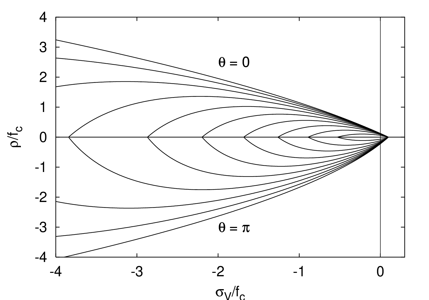
The yield surface is described in terms of the cylindrical coordinates in the principal effective stress space
(Haigh-Westergaard coordinates), which are the volumetric effective stress V = I1()∕3, the norm of the deviatoric
effective stress =  , and the Lode angle θ defined by the relation
| (146) |
where J2 and J3 are the second and third deviatoric invariants. The yield function
depends on the effective stress (which enters in the form of cylindrical coordinates) and on the hardening
variable κp (which enters through a dimensionless variable qh). Parameter c is the uniaxial compressive
strength. Note that, under uniaxial compression characterized by axial stress < 0, we have V = ∕3,
= - and = 60o. The yield function then reduces to fp = (∕c)2 - qh2. This means that function
qh describes the evolution of the uniaxial compressive yield stress normalized by its maximum value,
c.
and = 60o. The yield function then reduces to fp = (∕c)2 - qh2. This means that function
qh describes the evolution of the uniaxial compressive yield stress normalized by its maximum value,
c.
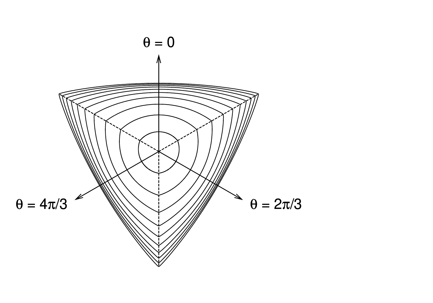
The evolution of the yield surface during hardening is presented in Fig. 9. The parabolic shape of the meridians (Fig. 9a) is controlled by the hardening variable qh and the friction parameter m0. The initial yield surface is closed, which allows modeling of compaction under highly confined compression. The initial and intermediate yield surfaces have two vertices on the hydrostatic axis but the ultimate yield surface has only one vertex on the tensile part of the hydrostatic axis and opens up along the compressive part of the hydrostatic axis. The deviatoric sections evolve as shown in Fig. 9b, and their final shape at full hardening is a rounded triangle at low confinement and almost circular at high confinement. The shape of the deviatoric section is controlled by the Willam-Warnke function
| (148) |
The eccentricity parameter e that appears in this function, as well as the friction parameter m0, are calibrated from the values of uniaxial and equibiaxial compressive strengths and uniaxial tensile strength.
| (a) | (b) |
 |  |
The maximum size of the elastic domain is attained when the variable qh is equal to one (which is its maximum value, as follows from the hardening law, to be specified in (153)). The yield surface is then described by the equation
| (149) |
The flow rule
| (150) |
is non-associated, which means that the yield function fp and the plastic potential
do not coincide and, therefore, the direction of the plastic flow ∂gp∕∂ is not normal to the yield surface. The ratio of the volumetric and the deviatoric parts of the flow direction is controled by function mg, which depends on the volumetric stress and is defined as
| (152) |
where Ag and Bg are model parameters that are determined from certain assumptions on the plastic flow in uniaxial tension and compression.
The dimensionless variable qh that appears in the yield function (147) is a function of the hardening variable κp. It controls the size and shape of the yield surface and, thereby, of the elastic domain. The hardening law is given by
| (153) |
The initial inclination of the hardening curve (at κp = 0) is positive and finite, and the inclination at peak (i.e., at κp = 1) is zero.
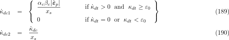
The evolution law for the hardening variable,3
| (154) |
sets the rate of the hardening variable equal to the norm of the plastic strain rate scaled by a hardening ductility measure
| (155) |
The dependence of the scaling factor xh on the volumetric effective stress V is constructed such that the model response is more ductile under compression. The variable
| (156) |
is a linear function of the volumetric effective stress. Model parameters Ah,Bh,Ch and Dh are calibrated from the values of strain at peak stress under uniaxial tension, uniaxial compression and triaxial compression, whereas the parameters
are determined from the conditions of a smooth transition between the two parts of equation (155) at Rh = 0.
For the present model, the evolution of damage starts after full saturation of plastic hardening, i.e., at κp = 1. This greatly facilitates calibration of model parameters, because the strength envelope is fully controled by the plastic part of the model and damage affects only the softening behavior. In contrast to pure damage models, damage is assumed to be driven by the plastic strain, more specifically by its volumetric part, which is closely related to cracking. To slow down the evolution of damage under compressive stress states, the damage-driving variable κd is not set equal to the volumetric plastic strain, but it is defined incrementally by the rate equation
| (159) |
where
| (160) |
is a softening ductility measure. Parameter As is determined from the softening response in uniaxial compression. The
dimensionless variable Rs =  pV -∕
pV -∕ pV is defined as the ratio between the “negative” volumetric plastic strain
rate
pV is defined as the ratio between the “negative” volumetric plastic strain
rate
| (161) |
and the total volumetric plastic strain rate  pV . This ratio depends only on the flow direction ∂gp∕∂, and thus Rs
can be shown to be a unique function of the volumetric effective stress. In (161),
pV . This ratio depends only on the flow direction ∂gp∕∂, and thus Rs
can be shown to be a unique function of the volumetric effective stress. In (161),  pI are the principal components of
the rate of plastic strains and
pI are the principal components of
the rate of plastic strains and  denotes the McAuley brackets (positive-part operator). For uniaxial tension, for
instance, all three principal plastic strain rates are nonnegative, and so
denotes the McAuley brackets (positive-part operator). For uniaxial tension, for
instance, all three principal plastic strain rates are nonnegative, and so  pV - = 0, Rs = 0 and xs = 1. This means
that under uniaxial tensile loading we have κd = κp - 1. On the other hand, under compressive stress
states the negative principal plastic strain rates lead to a ductility measure xs greater than one and the
evolution of damage is slowed down. It should be emphasized that the flow rule for this specific model is
constructed such that the volumetric part of plastic strain rate at the ultimate yield surface cannot be
negative.
pV - = 0, Rs = 0 and xs = 1. This means
that under uniaxial tensile loading we have κd = κp - 1. On the other hand, under compressive stress
states the negative principal plastic strain rates lead to a ductility measure xs greater than one and the
evolution of damage is slowed down. It should be emphasized that the flow rule for this specific model is
constructed such that the volumetric part of plastic strain rate at the ultimate yield surface cannot be
negative.
| Description | Damage-plastic model for concrete |
| Record Format | ConcreteDPM d(rn) # E(rn) # n(rn) # tAlpha(rn) # ft(rn) # fc(rn) # wf(rn) # Gf(rn) # ecc(rn) # kinit(rn) # Ahard(rn) # Bhard(rn) # Chard(rn) # Dhard(rn) # Asoft(rn) # helem(rn) # href(rn) # dilation(rn) # yieldtol(rn) # newtoniter(in) # |
| Parameters | - d material density |
| - E Young modulus |
|
| - n Poisson ratio | |
| - tAlpha thermal dilatation coefficient | |
| - ft uniaxial tensile strength ft |
|
| - fc uniaxial compressive strength |
|
| - wf parameter wf that controls the slope of the softening branch (serves for the evaluation of εf = wf∕h to be used in (162)) |
|
| - Gf fracture energy, can be specified instead of wf, it is converted to wf = Gf∕ft |
|
| - ecc eccentricity parameter e from (148), optional, default value 0.525 |
|
| - kinit parameter qh0 from (153), optional, default value 0.1 |
|
| - Ahard parameter Ah from (155), optional, default value 0.08 |
|
| - Bhard parameter Bh from (155), optional, default value 0.003 |
|
| - Chard parameter Ch from (155), optional, default value 2 |
|
| - Dhard parameter Dh from (155), optional, default value 10-6 |
|
| - Asoft parameter As from (160), optional, default value 15 |
|
| - helem element size h, optional (if not specified, the actual element size is used) |
|
| - href reference element size href, optional (if not specified, the standard adjustment of the damage law is used) |
|
| - dilation dilation factor (ratio between lateral and axial plastic strain rates in the softening regime under uniaxial compression), optional, default value -0.85 |
|
| - yieldtol tolerance for the implicit stress return algorithm, optional, default value 10-10 |
|
| - newtoniter maximum number of iterations in the implicit stress return algorithm, optional, default value 100 |
|
| Supported modes | 3dMat |
The relation between the damage variable ω and the internal variable κd (maximum level of equivalent strain) is assumed to have the exponential form
| (162) |
where εf is a parameter that controls the slope of the softening curve. In fact, equation (162) is used by the nonlocal version of the damage-plastic model, with κd replaced by its weighted spatial average (not yet available in the public version of OOFEM). For the local model, it is necessary to adjust softening according to the element size, otherwise the results would suffer by pathological mesh sensitivity. It is assumed that localization takes place at the peak of the stress-strain diagram, i.e., at the onset of damage. After that, the strain is decomposed into the distributed part, which corresponds to unloading from peak, and the localized part, which is added if the material is softening. The localized part of strain is transformed into an equivalent crack opening, w, which is under uniaxial tension linked to the stress by the exponential law
| (163) |
Here, ft is the uniaxial tensile strength and wf is the characteristic crack opening, playing a similar role to εf. Under uniaxial tension, the localized strain can be expressed as the sum of the post-peak plastic strain (equal to variable κd) and the unloaded part of elastic strain (equal to ωft∕E). Denoting the effective element size as h, we can write
| (164) |
and substituting this into (163), we obtain a nonlinear equation
| (165) |
from which the damage variable ω corresponding to the given internal variable κd can be computed by Newton iteration. The effective element size h is obtained by projecting the element onto the direction of the maximum principal strain at the onset of cracking, and afterwards it is held fixed. The evaluation of ω from κd is no longer explicit, but the resulting load-displacement curve of a bar under uniaxial tension is totally independent of the mesh size. A simpler approach would be to use (162) with εf = wf∕h, but then the scaling would not be perfect and the shape of the load-displacement curve (and also the dissipated energy) would slightly depend on the mesh size. With the present approach, the energy per unit sectional area dissipated under uniaxial tension is exactly Gf = wfft. The input parameter controling the damage law can be either the characteristic crack opening wf, or the fracture energy Gf. If both are specified, wf is used and Gf is ignored. If only Gf is specified, wf is set to Gf∕ft.
The onset of damage corresponds to the peak of the stress-strain diagram under proportional loading, when the ratios of the stress components are fixed. This is the case e.g. for uniaxial tension, uniaxial compression, or shear under free expansion of the material (with zero normal stresses). However, for shear under confinement the shear stress can rise even after the onset of damage, due to increasing hydrostatic pressure, which increases the mobilized friction. It has been observed that the standard approach leads to strong sensitivity of the peak shear stress to the element size. To reduce this pathological effect, a modified approach has been implemented. The second-order work (product of stress increment and strain increment) is checked after each step and the element-size dependent adjustment of the damage law is applied only after the second-order work becomes negative. Up to this stage, the damage law corresponds to a fixed reference element size, which is independent of the actual size of the element. This size is set by the optional parameter href. If this parameter is not specified, the standard approach is used. For testing purposes, one can also specify the actual element size, helem, as a “material property”. If this parameter is not specified, the element size is computed for each element separately and represents its actual size.
The damage-plastic model contains 15 parameters, but only 6 of them need to be actually calibrated for different concrete types, namely Young’s modulus E, Poisson’s ratio ν, tensile strength ft, compressive strength fc, parameter wf (or fracture energy Gf), and parameter As in the ductility measure (160) of the damage model. The remaining parameters can be set to their default values specified in [8].
The model parameters are summarized in Tab. 43. Note that it is possible to specify the “size” of finite element, h, which (if specified) replaces the actual element size in (165). The usual approach is to consider h as the actual element size (evaluated automatically by OOFEM), in which case the optional parameter h is missing (or is set to 0., which has the same effect in the code). However, for various studies of mesh sensitivity it is useful to have the option of specifying h as an input “material” value.
If the element is too large, it may become too brittle and local snap-back occurs in the stress-strain diagram, which is not acceptable. In such a case, an error message is issued and the program execution is terminated. The maximum admis sible element size
| (166) |
happens to be equal to Hillerborg’s characteristic material length. For typical concretes it is in the order of a few hundred mm. If the condition h < hmax is violated, the mesh needs to be refined. Note that the effective element size h is obtained by projecting the element. For instance, if the element is a cube of edge length 100 mm, its effective size in the direction of the body diagonal can be 173 mm.
This model is an extension of the ConcreteDPM presented in 1.6.9. CDPM2 has been developed by Grassl and coworkers for modelling the failure of concrete for both static and dynamic loading. It is is described in detail in [9]. The main differences between CDPM2 and ConcreteDPM are that in CDPM2
the plasticity part exhibits hardening once damage is active,
two independent damage parameters, which describe tensile and compressive damage, are introduced.
These extensions provide more flexibility, and the shapes of stress-strain curves under various loading scenarios, including unloading, can be better adapted. The price to pay is an increased number of parameters and thus more difficult calibration.
CDPM2 deals with the same definition of effective stress as ConcreteDPM, namely
| (167) |
which means that the effective stress is computed using the plastic part of the model. The effect of damage is incorporated in the transformation from effective to nominal stress. While ConcreteDPM uses a simple reduction factor 1 - ω (see (145)), CDPM2 splits the effective stress into the positive part, t, and the negative part, c, and then uses two damage variables, ωt and ωc (for tension and for compression). The nominal stress is thus evaluated as
| (168) |
The values of ωt and ωc range from 0 (undamaged) to 1 (fully damaged). The decomposition of the effective stress tensor into the positive and negative parts is based on principal values. If I, I = 1,2,3, are the principal effective stresses and nI, I = 1,2,3, are the corresponding principal directions, the effective stress tensor
| (169) |
is decomposed into
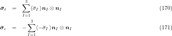
where ⟨…⟩ are Macaulay brackets (positive-part operator).
The yield condition is formulated in terms of the effective stress and therefore is unaffected by damage. The yield function is given by
| (172) |
where V is the volumetric effective stress, is the norm of the deviatoric effective stress and is the Lode angle (another invariant of the effective stress tensor). Parameter fc is the uniaxial compressive strength. Evolution of the yield surface is controlled by two dimensionless stress-like hardening variables, qh1 and qh2, which are considered as functions of one dimensionless strain-like hardening variable, κp. The hardening laws read
During the initial stage of hardening, κp grows from 0 to 1, qh1 grows from its initial value qh0 to 1 while qh2 remains equal to 1. No damage is induced and the yield surface is expanding. A change of behavior occurs when κp becomes equal to 1. For the original ConcreteDPM model, there would not be any further evolution of the yield surface. In CDPM2, linear hardening with constant plastic modulus Hp is assumed. Variable qh1 remains equal to 1 while qh2 grows proportionally to the increments of κp. If Hp is set to zero (i.e., qh2 remains equal to 1), the same behavior as for the ConcreteDPM is obtained.
The shape of the deviatoric section is controlled by the Willam-Warnke function
| (175) |
Here, e is the eccentricity parameter. The friction parameter m0 is given by
| (176) |
where ft is the tensile strength.
Hardening variable κp is a generalized form of cumulative plastic strain. Its rate corresponds to the rate of the norm of plastic strain rate scaled by a factor that depends on the stress state. This is described by the evolution equation
| (177) |
in which V is the hydrostatic part of effective stress and is the Lode angle. Function xh has a complicated form, designed such that κp grows faster for positive hydrostatic stress and more slowly under negative hydrostatic stress. Consequently, the material response is brittle in tension and less brittle or even ductile in compression, especially under confinement. The form of function xh suggested in [9] is
| (178) |
where
| (179) |
At the peak of the uniaxial compressive stress-strain curve, we have V = -fc∕3 and thus Rh = 0. Positive values of Rh correspond to confined compression. Under compression with no confinement, xh is equal to Bh, and under high confinement it is close to Ah. Parameter Ch controls the transition from Bh to Ah and if it is high, the transition occurs at higher compressive stresses. In this way, parameters Ah, Bh and Ch can be used to tune up the sensitivity of the model to confining stresses. Parameter Dh affects the behavior under combined tension and compression, or under uniaxial or multiaxial tension.
Parameters Eh and Fh are not considered as independent. To ensure a smooth transition between cases with positive and negative Rh, they need to be set to Eh = Bh - Dh and Fh = (Bh - Dh)Ch∕(Ah - Bh). Note that all these parameters are dimensionless. In [9] it was suggested to calibrate parameters Ah, Bh, Ch and Dh from the strains at peak stress under uniaxial tension, uniaxial compression and triaxial compression. Of course, four parameters cannot be uniquely determined from just three experimental values. It is desirable to use experimental data for triaxial compression at several levels of confinement. From the foregoing discussion of the role of individual parameters it follows that Ah should be greater than Bh, to obtain a positive effect of confinement on ductility, and parameter Dh should be smaller than Bh, to get a more brittle behavior in tension than in compression.
The flow rule is postulated in the non-associated format (150) with a plastic potential given by the same expression (151) as for the ConcreteDPM model, just with hardening variable qh formally replaced by qh1. The direction of plastic flow is given by the gradient of the plastic potential, and it can be split into the volumetric and deviatoric parts:
| (180) |
Taking into account that ∂V ∕∂ = δ∕3 and ∂∕∂ = ∕, restricting attention to the post-peak regime (in which qh1 = 1) and differentiating the plastic potential (151), we rewrite equation (180) as
| (181) |
Since the flow rule is non-associative, the direction of the plastic flow is not normal to the yield surface. This is important for concrete since an associative flow rule would give an overestimated maximum stress for passive confinement.
Damage is initiated when the equivalent strain reaches the threshold ε0 = ft∕E, which represents the limit elastic strain under uniaxial tension. The evolution of damage variables depends on certain internal variables linked to the elastic and plastic strains computed using the plastic part of the model.
The tensile damage variable ωt is a function of three auxiliary internal variables, κdt, κdt1 and κdt2. Variable κdt is the maximum previously reached value of equivalent strain
| (182) |
where r is the function of the Lode angle specified in (175) and m0 is the friction parameter specified in (176).
Expression (182) has been derived from the yield condition fp = 0 by setting qh1 = 1 and qh2 =  ∕ε0, which leads to a
quadratic equation.
∕ε0, which leads to a
quadratic equation.
Variables κdt1 and κdt2 are defined by the rate equations
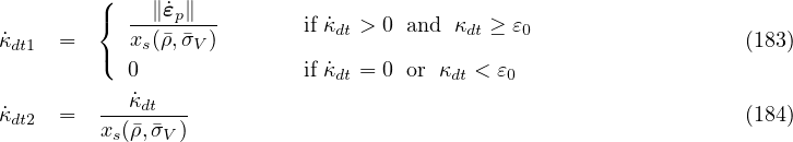
where
| (185) |
is a ductility measure. For positive hydrostatic stress V , we have ⟨-V ⟩ = 0 and xs = 1. Under compression, xs
increases (provided that parameter As is greater than 1), which slows down the evolution of variables κdt1 and κdt2
and consequently of damage. For uniaxial compression, we have V ∕ = -1∕ and formula (185) gives
xs = As.
and formula (185) gives
xs = As.
The specific form of the dependence of damage variable ωt on κdt, κdt1 and κdt2 is dictated by the desired shape of the softening part of the uniaxial tensile stress-strain diagram. For instance, bilinear softening is obtained with
| (186) |
where εf1 and σ1 is the strain and stress at the knee point of the softening diagram (where the two linear segments meet), and εf is the strain at which the stress vanishes. The choice of a bilinear softening diagram for tension makes it possible to obtain a steep initial descent followed by a long tail, which would not be that easy with the exponential diagram used in the ConcreteDPM model. In the local version of the model, objectivity with respect to mesh size must be enforced by adjustment of the softening diagram. Numerical parameters εf1 and εf are then derived from material parameters wf1 and wf that define the cohesive law in terms of the dependence of stress on crack opening, w. Transformation of crack opening into the smeared cracking strain then leads to parameters εf1 = wf1∕h and εf = wf∕h where h is the estimated thickness of the computationally resolved localized band.
The compressive damage variable ωc is a function of three auxiliary internal variables, κdc, κdc1 and κdc2. Variable κdc is defined by the rate equation
| (187) |
where  is the already defined equivalent strain, and the scaling factor αc depends on the type of stress state and is
given by
is the already defined equivalent strain, and the scaling factor αc depends on the type of stress state and is
given by
| (188) |
If all principal effective stresses σI are positive (or at least non-negative), we have αc = 0, and if all principal effective stresses are negative (or at least non-positive), we have αc = 1. For the zero stress state, αc is undefined, but for that particular state it is not needed.
Two other auxiliary internal variables that affect compressive damage are defined by the rate equations
where factor
| (191) |
depends on the plastic hardening variable qh2 and effective stress invariant and provides a smooth transition from pure damage to damage-plastic softening, which can occur during cyclic loading. The dependence of the compressive damage ωc on the internal variables is defined such that the relation between the stress and the inelastic strain, εi, under uniaxial compression is exponential and is given by
| (192) |
where εfc is a parameter controls the initial inclination of the softening curve. The inelastic strain is defined as the difference between the total strain, ε, and the elastic strain, σ∕E. Replacing σ bythe right-hand side of (192), we obtain a nonlinear equation
| (193) |
from which εi can be evaluated iteratively if the total strain ε is given. The use of different damage evolution rules for tension and compression is one important improvement over ConcreteDPM. In contrast to tension, the evolution law for compressive damage is considered to be independent of the element size, since compressive failure is often characterized by mesh-independent zones of damage growth.
| parameter | OOFEM | unit | default | meaning |
| identifier | value | |||
| E | E | Pa | Young’s modulus | |
| ν | n | - | Poisson’s ratio | |
| ft | ft | Pa | uniaxial tensile strength | |
| fc | fc | Pa | uniaxial compression strength | |
| wf | wf | m | critical crack opening | |
| e | ecc | - | 0.525 | eccentricity, eq. (175)–(176) |
| qh0 | kinit | - | 0.3 | initial value of hardening variable qh1, eq. (173) |
| Hp | hp | - | 0.5 | hardening modulus (for the last stage, eq. (174)) |
| Df | dilation | - | 0.85 | dilation factor, eq. (191) |
| Ah | Ahard | - | 0.08 | hardening parameter, eq. (178) |
| Bh | Bhard | - | 0.003 | hardening parameter, eq. (178) |
| Ch | Chard | - | 2 | hardening parameter, eq. (178) |
| Dh | Dhard | - | 10-6 | hardening parameter, eq. (178) |
| As | Asoft | - | 15 | softening parameter, eq. (161) |
| εfc | efc | - | 10-4 | softening parameter for compression, eq. (192) |
| stype | 1 | type of softening (1=bilinear) | ||
| wf1∕wf | wf1 | - | 0.15 | softening parameter for tension |
| σ1∕ft | ft1 | - | 0.3 | softening parameter for tension, eq. (186) |
From the presented description of the model equations, it is clear that CDPM2 uses a large number of parameters. In [9] it was recommended to adjust only a few basic parameters, most of which have a certain physical meaning, and to set all the other parameters to their default values. The physical parameters that can be adjusted depending on the specific type of concrete are Young’s modulus, Poisson’s ratio, uniaxial tensile and compression strengths, and the critical crack opening, which controls the tensile fracture energy. A summary of all model parameters and of their recommended default values is provided in Table 44. The table shows the symbol used for the parameter in equations describing the theoretical background and also the corresponding identifier used in OOFEM input files.
Parameters listed on the first five lines of Table 44 must be specified by the user. Parameter wf corresponds to the opening of a cohesive crack at which the stress transmitted by the crack vanishes. It is closely related to the tensile fracture energy, GFt. The shape of the cohesive curve for tensile failure is affected by the choice of the type of softening. The default choice is bilinear softening, which requires, in addition to ft and wf, two more parameters that control the position of the point at which the slope of the diagram changes. This point is characterized by crack opening wf1 and stress σ1, but the input parameters for OOFEM are dimensionless ratios wf1∕wf and σ1∕ft with default values 0.15 and 0.3. In general, the fracture energy is evaluated as GFt = (ftwf1 + σ1wf)∕2, and for the default values this gives GFt = ftwf∕4.444, which means that parameter wf can be evaluated from the tensile strength and fracture energy using formula wf = 4.444GFt∕ft.
The eccentricity parameter e could be evaluated from ft and fc combined with the biaxial compression strength, fbc, using formula
| (194) |
where
| (195) |
The default value is not mentioned in [9]; in OOFEM it is taken as e = 0.525.
Parameter Hp is a dimensionless hardening modulus that sets the ratio between the increments of variables qh2 and κp during the last stage of the plastic hardening process. The value recommended in [9] is Hp = 0.01, but the default value used in OOFEM is 0.5.
The dilation parameter Df controls the ratio between the transversal and axial plastic strain rates in uniaxial compression and thus can be used to control the volumetric expansion in the softening regime. The default value is set to 0.85, as suggested in [8], which means that the transversal plastic strain rate will be -0.85 times the (negative) axial plastic strain rate.
The default values of qh0 = 0.3, Ah = 0.08, Bh = 0.003, Ch = 2, Dh = 10-6 and εfc = 10-4 are taken from [9]. Parameter As was varied in [9] in the range from 1.5 to 15. In OOFEM, the default value of As is taken as 15, which was recommended in [8].
Concrete is strongly rate-dependent. If the loading rate is increased, the tensile and compressive strength increase and are more prominent in tension then in compression. The dependency of the stress-strain response on the dynamic increase factor is taken into account by an additional variable αr. The rate dependency is included by scaling both the equivalent strain rate and the inelastic strain. The rate parameter is defined by
| (196) |
where X is the continuous compression measure (= 1 means only compression, = 0 means only tension). The dynamic increase factor (DIF) for strength is computed according to Model Code 2010.
The parameters of CDPM2 for OOFEM input file are summarised in Tab. 45. By default, two damage variables are used, i.e., the effective stress is transformed into nominal stress using equation (168). If parameter damflag is set to 3, only ωt is used and the effective stress is reduced by 1 - ωt.
| Description |
CDPM2 |
| Record Format |
con2dpm d(rn) # E(rn) # n(rn) # tAlpha(rn) # ft(rn) # fc(rn) # wf(rn) # [stype(in) #] [ft1(rn) #] [wf1(rn) #] [efc(rn) #] [ecc(rn) #] [kinit(rn) #] [Ahard(rn) #] [Bhard(rn) #] [Chard(rn) #] [Dhard(rn) #] [Asoft(rn) #] [helem(rn) #] [dilation(rn) #] [hp(rn) #] [damflag(in) #] [sratetype(in) #] eratetype(in) # [yieldtol(rn) #] [newtoniter(in) #] |
| Parameters |
- d material density |
|
- E Young modulus |
|
|
- n Poisson ratio |
|
|
- tAlpha thermal dilatation coefficient |
|
|
- ft uniaxial tensile strength |
|
|
- fc uniaxial compressive strength |
|
|
- wf parameter that controls the slope of the softening branch to be used |
|
|
- stype allows to choose different types of softening laws, default value 1:
|
|
|
- ft1 parameter for the bilinear softening law (stype = 1) defining the ratio between intermediate stress and tensile strength, optional, default value 0.3 |
|
|
- wf1 parameter for the bilinear softening law (stype = 1) defining the intermediate crack opening, optional, default value 0.15 |
|
|
- efc parameter for exponential softening law in compression, optional, default value 100 × 10-6 |
|
|
- ecc eccentricity parameter, optional, default value 0.525 |
|
|
- kinit initial value of hardening law, optional, default value 0.3 |
|
|
- Ahard hardening parameter, optional, default value 0.08 |
|
|
- Bhard hardening parameter, optional, default value 0.003 |
|
|
- Chard hardening parameter, optional, default value 2 |
|
|
- Dhard hardening parameter, optional, default value 1 × 10⁻⁶ |
|
|
- Asoft softening parameter, optional, default value 15 |
|
|
- helem element size h, optional (if not specified, the actual element size is used) |
|
|
- dilation dilation factor, optional, default value 0.85 |
|
|
- hp hardening modulus, optional, default value 0.5 |
|
|
- damflag flag which allows for the use of different damage formulations. Default value is 1. If set to zero, no damage is used. If set to 3, only the tensile damage varialbe is used. |
|
|
- sratetype Dynamic increase factor (DIF) for strength
|
|
|
- eratetype Dynamic increase factor (DIF) for fracture energy. Only used if sratetype is not equal to 0.
|
|
|
- yieldtol tolerance for the implicit stress return algorithm, optional, default value 1 × 10⁻⁶ |
|
|
- newtoniter maximum number of iterations in the implicit stress return algorithm, optional, default value 100 |
|
| Supported modes |
3dMat, PlaneStrain, 1dMat |
Implementation of a fixed crack model. Uncracked material is modeled as isotropic linear elastic characterized by Young’s modulus and Poisson’s ratio. Cracking is initiated when principal stress reaches tensile strength. Further loading is governed by a softening law. Proper amount energy dissipation is guaranteed by the crack-band approach. Multiple cracking is allowed; the maximum number of allowed cracks is controlled by ncracks parameter. Only mutually perpendicular cracks are supported. If cracking occurs in more directions, the behavior on the crack planes is considered to be independent. The secant stiffness is used for unloading and reloading. In a compression regime, this model correspond to an isotropic linear elastic material. The model supports 3 different options for stiffness reduction in shear after cracking, 2 options for the limit of the maximum shear stress on a crack plane and 6 different laws for postpeak behavior. The model parameters are summarized in Tab. 46.
Sample syntax for a fixed crack model with volume density 24 kN/m3, thermal dilation coefficient 12 × 10-6 K-1,
Young’s modulus 20 GPa, Poisson’s ratio 0.2, fracture energy 100 N/m, tensile strength 2 MPa, linear softening,
constant shear retention factor β = 0.05, Collins’ shear strength (with compressive strength 30 MPa,
aggregate size 0.01 m) and all cracks contribute to the shear stiffness; the analysis uses [m], [MPa] and
[MN]:
ConcreteFCM 1 d 24.e-3 talpha 12.e-6 E 20000. n 0.2 Gf 100e-6 ft 2.0 softType 2 shearType 1 beta
0.05 shearStrengthType 2 fc 30 ag 0.01
lengthscale 1. multipleCrackShear
| Description |
Fixed crack model for concrete |
| Record Format |
ConcreteFCM (in) # d(rn) # tAlpha(rn) # E(rn) # n(rn) # [ ncracks(in) #] [ multipleCrackShear ] [ crackSpacing(rn) #] [ softType(in) #] [ shearType(in) #] [ shearStrengthType(in) #] [ ecsm(rn) #] [ Gf(rn) #] [ ft(rn) #] [ beta(rn) #] [ sf(rn) #] [ fc(rn) #] [ ag(rn) #] [ lengthscale(rn) #] [ soft_w(ra) #] [ soft(w)(ra) #] [ soft_eps(ra) #] [ soft(eps)(ra) #] [ beta_w(ra) #] [ beta(w)(ra) #] [ H(rn) #] [ eps_f(rn) #] |
| Parameters |
- material model number |
|
- d material density |
|
|
- tAlpha thermal dilatation coefficient |
|
|
- E Young’s modulus |
|
|
- n Poisson’s ratio |
|
|
- ncracks maximum allowed number of cracks |
|
|
- crackSpacing specified distance between parallel cracks |
|
|
- multipleCrackShear if not given, shear stiffness computed from the dominant crack, otherwise all cracks contribute |
|
|
- softType allows to select suitable softening law:
|
|
|
- shearType offers to choose from different approaches for shear stiffness reduction of a cracked element
|
|
|
- shearStrengthType allows to select a shear stress limit on a crack plane
|
|
|
- ecsm method used for evaluation of characteristic element size L: 1 = square root of area, 2 = projection centered, 3 = Oliver, 4 = Oliver modified, 0 (default) = projection |
|
|
- Gf fracture energy |
|
|
- ft tensile strength |
|
|
- beta shear retention factor |
|
|
- sf shear factor coefficient |
|
|
- fc compressive strength in MPa |
|
|
- ag aggregate size |
|
|
- lengthscale factor to convert crack opening and aggregate size in case of Collins aggregate interlock; 1 = analysis in meters, 1000 = in millimeters, etc. |
|
|
- soft_w specified values of crack opening and |
|
|
- soft(w) corresponding values of traction normalized to ft |
|
|
- soft_eps specified values of cracking strain and |
|
|
- soft(eps) corresponding values of traction normalized to ft |
|
|
- beta_w specified values of crack opening and |
|
|
- beta(w) corresponding values of shear retention factor |
|
|
- H hardening modulus (expressed wrt cracking strain) |
|
|
- eps_f threshold for cracking strain after which traction is zero (applicable for linear hardening only) |
|
| Supported modes |
3dMat, PlaneStress, PlaneStrain |
The material model “ConcreteFcmViscoelastic” has been developed in order to realistically capture the time-dependent behavior of cementitious materials with the possibility of tensile cracking. The model allows to link an arbitrary viscoelastic material model present in OOFEM with the model ”ConcreteFCM” for tensile failure with fixed (not rotating) orientation of cracks developed for concrete. The material model assumes an additive split of the total deformation into the viscoelastic and cracking part. The viscoelastic material handles the stress-independent strains, i.e. shrinkage and thermal dilation.
In the case of an elastic (initial) stiffness or uncracked material, the stiffness matrix ve is evaluated as the product of incremental stiffness of the viscoelastic material and the unit elastic stiffness matrix Dv. The evaluation of the incremental modulus is computationally demanding, therefore within one time step it is stored in the material status. The value of stiffness depends on the history of relative humidity and temperature at given Gauss point and depends entirely on the viscoelastic material.
Secant stiffness matrix is obtained by adding the secant compliance of the cohesive cracks to the viscoelastic compliance matrix and by subsequent inversion of the result.
| (197) |
Tangent stiffness matrix is computed as
| (198) |
where Dcr is the tangent stiffness of the cracked material.
The secant and tangent matrix are constructed in the local coordinate system corresponding to the orientation of the cracks and then are rotated to the global coordinate system. The individual components of Dcr are managed by ConcreteFCM material model.
The stress evaluation algorithm can be decomposed into 3 subsequent steps:
Call the viscoelastic material to compute the stress-dependent strain increment
| (199) |
where Δε is the total strain increment, Δε′′ is the strain increment due to creep, Δεsh is the shrinkage increment, and ΔεT is the thermal dilation increment.
Call the fixed-crack material to compute the new stress vector σi+1 fulfilling the nonlinear equation
| (200) |
where σi is the old stress vector and Δεcr is the increment of crack strain, and update the new crack strain vector
| (201) |
Pass the difference of the total strain and the cracking strain to the viscoelastic material and perform a regular viscoelastic step.
| (202) |
Before the onset of cracking, the material is modeled as isotropic linear viscoelastic characterized by its compliance function, Poisson’s ratio, and the evolution of shrinkage which can depend both on equivalent time and change in relative humidity provided that the problem is solved as coupled.
Cracking is initiated when principal stress reaches tensile strength. Further loading is governed by a softening law. Proper amount energy dissipation is guaranteed by the crack-band approach, the width of the crack band is given by the size of the finite element projected in the direction of the principal stress.
Multiple cracking is allowed, the maximum number of cracks is controlled by ncracks parameter. Only mutually perpendicular cracks are supported. If cracking occurs in more directions, the behavior on the crack planes is considered to be independent. The secant stiffness is used for unloading and reloading. In compression regime full stiffness is restored.
It is worth emphasizing that the status of the viscoelastic material tracks and keeps only a part of the total deformation equal to the difference of the total strain and the cracking strain.
The current implementation supports both constant and time-evolving values of tensile strength and fracture energy. Constant values are used when the keyword timeDepFracturing is missing in the definition of the material. Then, the values are taken directly from the ConcreteFCM material (keywords ft and gf). On the other hand, when the flag timeDepFracturing is present in the material definition, the tensile strength and fracture energy is time-evolving. In that case, the values of ft and gf are ignored, and the value of parameter s (fib_s), and the mean value of the compressive strength fcm,28 (fcm28) need to be provided and serve for the prediction of ft(t) and GF(t). Yet, it is possible to override the predicted 28-day values by providing the fields ft28 and gf28. It must be noted that once the tensile stress exceeds the current value of tensile strength, the time development of the properties is terminated on the particular crack plane.
Mean value of the uniaxial compressive strength at specific time which is used for evaluation of the tensile strength and fracture energy is computed using expressions (5.1-50) and (5.1-51) in fib MC2010 [32]:
| (203) |
in which s is a coefficient reflecting cement type (table 5.1-9), te is the equivalent time from the viscoelastic model, and fcm,28 is the mean value of the uniaxial compressive strength at the age of 28 days.
Current value of tensile strength fctm(t) at time t is computed from the compressive strength at corresponding age, similarly to section 5.1.5.1 in MC2010. The difference is that in MC2010 both tensile strength and fracture energy are treated as non-aging and are evaluated from fcm,28. In the following expressions the fcm and fctm are in MPa.
| (204) |
| (205) |
| (206) |
The value of fracture energy at the age of 28 days is computed accordingly to section 5.1.5.2 in MC2010
| (207) |
in this equation GF is in N/m and the compressive strength is in MPa. Here, the time development of fracture energy is chosen to be the same as the tensile strength
| (208) |
| Description |
Viscoelastic fixed crack model for concrete |
| Record Format |
ConcreteFCMViscoelastic viscoMat(in) # gf(rn) # ft(rn) # [ timeDepFracturing ] [ fib_s(rn) #] [ fcm28(rn) #] [ timefactor(rn) #] [ stiffnessfactor(rn) #] [ gf28(rn) #] [ ft28(rn) #] |
| Parameters |
- material model number |
|
- viscoMat number of the slave viscoelastic material |
|
|
- ft tensile strength - constant value |
|
|
- gf fracture energy - constant value |
|
|
- timeDepFracturing flag to activate evolving ft and Gf according to fib MC2010 |
|
|
- fib_s strength class of cement coefficient (Table 5.1-9 in fib MC2010) |
|
|
- fcm28 28-day mean compressive strength of concrete used for prediction and evolution of ft and Gf |
|
|
- timefactor time transformation factor, 1 for days, 86400 for seconds etc. |
|
|
- stiffnessfactor stiffness transformation factor, 1 for Pa, 1.e6 for MPa etc. |
|
|
- ft28 overrides predicted tensile strength |
|
|
- gf28 overrides predicted fracture energy |
|
| Supported modes |
3dMat, PlaneStress, PlaneStrain |
The following lines show a sample syntax specifying the viscoelastic fixed crack model with the compliance defined by
the MPS model. Volume density is 24 kN/m3, thermal dilation coefficient 12 × 10-6 K-1, Poisson’s ratio 0.2, fracture
energy Gf and tensile strength ft predicted from the mean compressive strength fcm = 30 MPa (defined ft and gf are
discarded, to override use keywords ft28 and gf28), exponential softening, maximum 2 perpendicular tensile cracks,
constant shear factor coefficient, sf = 20., all cracks contribute to the shear stiffness, shear strength equal to ft,
numerical stiffness factors 1e-3, number of viscoelastic material is 2. The analysis uses [m], [MPa], [MN], and
[day]:
ConcreteFcmViscoelastic 1 d 24.e-3 talpha 0. E 30000. n 0.2
Gf 100.e-6 ft 2. softtype 1 sheartype 2 sf 20.
multiplecrackshear shearstrengthtype 1 ncracks 2
shearCoeffNumer 0.001 normalCoeffNumer 0.001 viscomat 2
timeDepFracturing fib_s 0.20 fcm28 30. timeFactor 1.
stiffnessFactor 1.e6
The viscoelastic material can be defined e.g. by the following listing. Note that the coefficient of thermal expansion is zero in ConcreteFcmViscoelastic and nonzero in the viscoelastic material which handles all stress-independent strains. Also note same values of the Poisson’s ratio.
mps 2 d 24.e-3 n 0.2 talpha 12.e-6 referencetemperature 296.
mode 0 fc 30. cc 340. w/c 0.523 a/c 5.28 stiffnessfactor 1.e6
timefactor 1. lambda0 1. begoftimeofinterest 1.e-6
endoftimeofinterest 1.e4 relMatAge 7. CoupledAnalysisType 2
ksh 0.0 k3 35. p 1000.
This material model is an extension of the ConcreteFCM described in Section 1.6.11.
It is possible to choose from three different “classes” of fibers. This choice is controlled by keyword fiberType: 0 = continuous aligned fibers (CAF), 1 = short aligned fibers (SAF) and 2 = short random fibers (SRF). Currently, it is not possible to combine more classes of fibers in one material model.
All of the above-mentioned fiber types are further defined by the material properties and geometry. Fiber quantity is captured by the dimensionless volume fraction Vf (as decimal). All fibers are assumed to have a circular cross-section (shape factor for shear kfib with default value 0.9) and to possess the same geometry characterized by the diameter Df and length Lf.
The overall elastic stiffness of the fiber-reinforced composite is calculated as a weighted average of the moduli of matrix Em and fibers Ef and the Poisson’s ratio is considered to be equal to the Poisson’s ratio of the matrix. Similarly to ConcreteFCM, cracking is initiated once the tensile stress σ in matrix reaches the tensile strength ft.
The nominal bridging stress for continuous aligned fibers which are not perpendicular to the crack plane σb,f,θ can be very easily obtained by multiplying the nominal bridging stress for perpendicular fibers σb,f by two terms: the first one reflecting lower volume of inclined fibers passing through the crack plane and the second one capturing the snubbing effect:
| (209) |
where f is a snubbing coefficient.
For the CAF perpendicular to the crack, the nominal bridging stress can be derived as
| (210) |
where η = (EfV f)∕[Em(1 - V f)].
For SRF the nominal bridging stress is
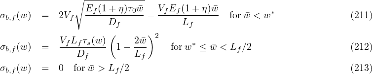
where w* =  ∕[(1 + η)EfDf]; τ0 is the bond shear strength between the fiber and matrix for small crack
openings, w < w*.
∕[(1 + η)EfDf]; τ0 is the bond shear strength between the fiber and matrix for small crack
openings, w < w*.
Larger pull-out displacements can lead to significant physical changes in the fiber surface which can result into changes in the bond shear stress. This phenomenon is captured by function τs(w) relating the frictional bond to the crack opening and is implemented in three alternative formulations. (In order to keep τs(w) = τ0 use fssType = 0.) In conventional FRC with ordinary concrete matrix, the frictional bond usually decreases with increasing slip. To capture this type of behavior we adopt the function proposed by Sajdlová (activated with fssType = 1) reads
| (214) |
where b0 is a micromechanical parameter. In composites with high-strength matrix and coated high-strength steel fibers (HSFRC, UHPFRC) as well as in SHCC materials with polymeric fibers, the frictional bond-slip relation often exhibits hardening; this phenomenon can be well approximated by a cubic function (activated with fssType = 2) proposed by Kabele
| (215) |
or an alternative formulation which results in smooth changes in the bridging stress (activated with fssType = 3)
| (216) |
In the last two equations b1, b2 and b3 are micromechanical parameters and additionally in the last equation
 = w - w*,
  = τ0(1. - w*∕Lf)-2 for SRF and
  = τ0Ef(1 + η)Df∕[Ef(1 + η)Df - 2Lfτ0] for
SAF.
= τ0Ef(1 + η)Df∕[Ef(1 + η)Df - 2Lfτ0] for
SAF.
The bridging stress for SRF is defined as
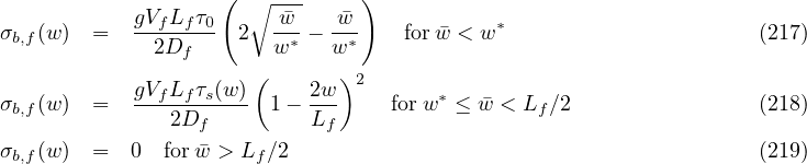
where g is the snubbing factor is defined as
| (220) |
It is possible to delay the activation of the stress in fibers using prameteter fibreActivationOpening which can be imagined as a “lag” of the fiber-related crack opening behind the matrix-related crack opening.
During unloading the stress in fibers does not decrease linearly to origin. Current implementation uses a power function
| (221) |
where wmax is the maximum crack width reached in the entire previous history and M is a positive constant, its default value is M = 4.
The influence of crack opening and sliding on the bridging shear stress only due to fibers is expressed as
| (222) |
where f is the effective volume of fibers crossing a crack plane (V f∕2 for SRF and V f cos(θ) for CAF and SAF), and Gf is the fiber shear modulus. This expression is motivated by assumption that the fibers bridging the crack planes behave as the Timoshenko beams subjected to shear. Note that the shear stiffness of fibers is not recovered upon unloading.
It has been found that in some high performance fiber reinforced cement composites, fibers rupture when cracks are exposed to shearing. This phenomenon is modeled by damage parameter ω, which accounts for the ratio of ruptured fibers and varies between the values of 0 and 1. It is assumed that ω depends on the maximum shear strain sustained by the protruding portions of bridging fibers throughout the loading history. This crack shear strain can be expressed as:
| (223) |
where ui is the crack sliding displacement (CSD) and and wi is the maximum value of the crack opening displacement of the i-th crack. This means that the damage does not grow if the crack closes (crack opening decreases). If more cracks exist, the maximum contribution is considered.
Two different one-parameter damage evolution laws are currently implemented. For fDamType = 0 the damage is deactivated, with fDamType = 1 damage is described by
| (224) |
and finally with fDamType = 2
| (225) |
where γfc (gammaCrack in the input record) is a parameter.
Since damage reduces the number of crack-bridging fibers, which is proportional to the fiber volume fraction, its effect can be suitably implemented by introducing the effective volume fraction
| (226) |
The material parameters are summarized in Tables 46 (matrix) and 48 (fiber extension).
Sample syntax for a fixed crack model reinforced with fibers with volume density 24 kN/m3, thermal dilation
coefficient 12 × 10-6 K-1, Young’s modulus of the matrix 20 GPa, Poisson’s ratio of matrix 0.2, fracture energy of
matrix 100 N/m, tensile strength of matrix 2 MPa, linear tension softening, constant shear retention factor β = 0.05,
unlimited shear strength (shearStrengthType = 0), continuous aligned fibers, fiber volume 2%, fiber
diameter 0.04 mm, Young’s modulus of fibers 20 GPa, shear modulus of fibers 1 GPa, fiber-matrix bond
strength 1 MPa, snubbing coefficient 0.7, shear correction coefficient 0.9, deactivated fiber damage, fiber
act if COD exceeds 10 μm (with smoothing from w = 8to11 μm), fiber orientation at 45 degrees in
x-y plane, automatic evaluation of crack spacing from composition; the analysis uses [m], [MPa] and
[MN]:
FRCFCM 1 d 24.e-3 talpha 12.e-6 E 20000. n 0.2 Gf 100e-6 ft 2.0
softType 2 shearType 1 beta 0.05 FiberType 0 Vf 0.02 Df 0.04e-3
Ef 20000. Gfib 1000. tau_0 1. FSStype 0 f 0.7 kfib 0.9 fDamType 0
fibreactivationopening 10.e-6 dw0 2.e-6 dw1 1.e-6 orientationVector 3 1. 1. 0. computeCrackSpacing
| Description |
Fixed crack model for FRC |
| Record Format |
FRCFCM input record of ConcreteFCM Vf(rn) # Lf(rn) # Df(rn) # Ef(rn) # [ nuf(rn) #] [ Gfib(rn) #] [ kfib(rn) #] tau_0(rn) # b0(rn) # b1(rn) # b2(rn) # b3(rn) # f(rn) # [ M(in) #] [ fibreOrientationVector(ra) #] [ fssType(in) #] [ fDamType(in) #] [ fiberType(in) #] [ gammaCrack(rn) #] [ computeCrackSpacing ] [ fibreActivationOpening(rn) #] [ dw0(rn) #] [ dw1(rn) #] |
| Parameters |
- Vf fiber content expressed as decimal |
|
- Lf fiber length |
|
|
- Df fiber diameter |
|
|
- Ef fiber Young’s modulus |
|
|
- nuf fiber Poisson’s ratio |
|
|
- Gfib fiber shear modulus (read when nuf is not provided) |
|
|
- kfib fiber cross-sectional shape correction factor |
|
|
- tau_0 bond shear strength at zero slip |
|
|
- b0 micromechanical parameter for fiber shear according to Sajdlová |
|
|
- b1, b2, b3 micromechanical parameter for fiber shear according to Kabele |
|
|
- f snubbing friction coefficient |
|
|
- M exponent related to fiber unloading |
|
|
- fibreOrientationVector vector specifying orientation for CAF and SAF fibers |
|
|
- fssType type of Fiber bond Shear Strength (bond shear strength vs. crack opening)
|
|
|
- fDamType type of damage law for fibers
|
|
|
- fiberType type of reinforcing fibers
|
|
|
- gammaCrack crack shear strain parameter applicable with fDamType = 1 or 2 (here the crack shear strain is understood as the crack slip u divided by the crack opening w) |
|
|
- computeCrackSpacing crack spacing is evaluated automatically based on provided composition |
|
|
- fibreActivationOpening crack opening at which the fibers begin transferring bridging stress |
|
|
- dw0, dw1 applicable only if fibreActivationOpening ≠0, then it allows to smooth the traction-separation law for fibers; lower bound is fibreActivationOpening - dw0 and the upper bound is fibreActivationOpening - dw1 |
|
| Supported modes |
3dMat, PlaneStress, PlaneStrain |
The material parameters are summarized in Tables 46 (matrix), 48 (fiber extension), and 49 (nonlocal extension).
| Description |
Nonlocal fixed crack model for FRC |
| Record Format |
FRCFCMNL input record of ConcreteFCM and FRCFCM r(rn) # wft(in) # |
| Parameters |
- r nonlocal radius (reasonable value is several millimeters and its maximum is Lf∕2 for short fibers) |
|
- wft nonlocal averaging function, must be set to 4 (constant function) |
|
| Supported modes |
PlaneStress |
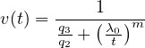
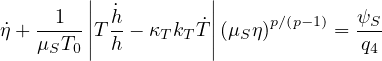
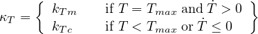
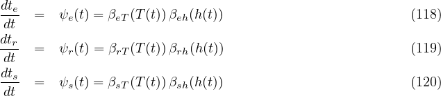
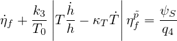

![[ ( )w∕c∕0.38] -4.5
εsh,au,B4(te) = ε∞sh,au,B4 1+ τau
te](matlibmanual186x.png)


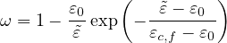


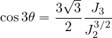
![( ( )2 ∘-- )2
f (σ¯ ,¯ρ,θ¯;κ ) = [1 - q(κ )] √-¯ρ--+ σ¯V- + 3ρ¯ +
p V p h p 6¯fc ¯fc 2f¯c
( ¯ρr(¯θ) ¯σ )
+m0q2h(κp) √--¯-+ ¯V- - q2h(κp) (147)
6fc fc](matlibmanual205x.png)
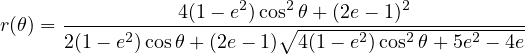
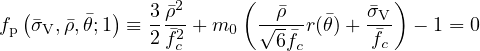

![( ( )2 ∘ -- )2
gp(¯σV, ¯ρ;κp) = [1 - qh(κp)] √¯ρ--+ ¯σ¯V- + 3-¯ρ¯ +
6¯fc fc 2fc
2 (-m0¯ρ- mg-(σ¯V-))
+q h(κp) √6-¯fc + ¯fc (151)](matlibmanual210x.png)
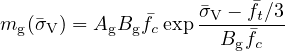
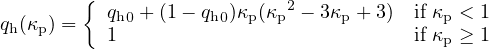
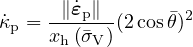
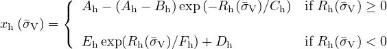
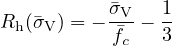
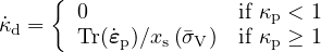
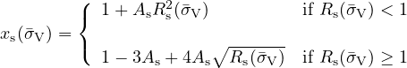
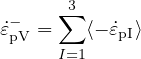
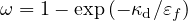

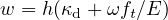
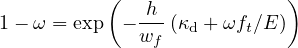
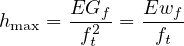
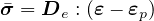

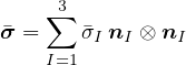
![{ ( )2 ∘ -- }2
f (¯σ ,¯ρ,¯θ;κ ) = [1- q (κ )] √¯ρ--+ ¯σV- + 3-¯ρ
p V p h1 p 6fc fc 2fc
[ ¯ρ ¯σ ]
+ m0q2h1(κp)qh2(κp) √---r(cos ¯θ) + -V- - qh21(κp)q2h2(κp)
6fc fc](matlibmanual235x.png)
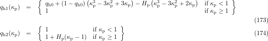

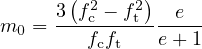
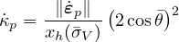

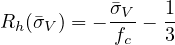
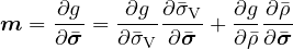
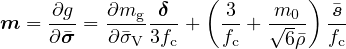
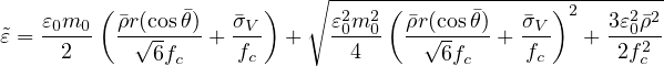
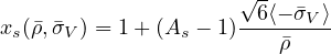
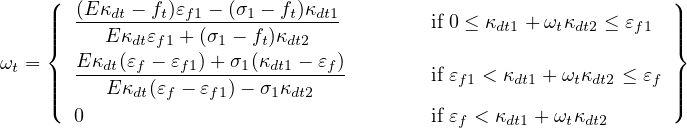

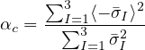
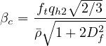
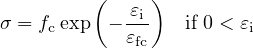
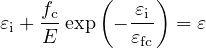

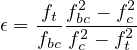

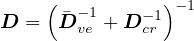


![[ ( ∘ ----)]
fcm(te) = exp s 1.- 28∕te fcm,28](matlibmanual266x.png)


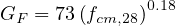
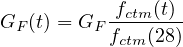

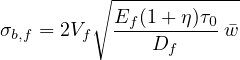
![[ ( ( ) )]
τs(w) = τ0 1+ sign(b0) 1 - exp - |b0|w-
Df](matlibmanual276x.png)
![[ ]
w ( w )2 ( w )3
τs(w) = τ0 1+ b1D--+ b2 D-- + b3 D--
f f f](matlibmanual277x.png)
![[ ( ) ( ) ]
-˜w- -˜w- 2 -˜w- 3
τs(w) = ˜τ0 + τ0 b1Df + b2 Df + b3 Df](matlibmanual278x.png)