1.5 Material models for tensile failure
1.5.1 Nonlinear elasto-plastic material model for concrete plates and shells - Concrete2
The description can be found is section 1.4.8.
1.5.2 Smeared rotating crack model - Concrete3
Implementation of smeared rotating crack model. Virgin material is modeled as isotropic linear elastic material
(described by Young modulus and Poisson ratio). The onset of cracking begins, when principal stress reaches tensile
strength. Further behavior is then determined by softening law, governed by principle of preserving of fracture energy
Gf. For large elements, the tension strength can be artificially reduced to preserve fracture energy. Multiple
cracks are allowed. The elastic unloading and reloading is assumed. In compression regime, this model
correspond to isotropic linear elastic material. The model description and parameters are summarized in
Tab. 22.
|
|
| Description | Rotating crack model for concrete |
|
|
|
Record Format | Concrete3 d(rn) # E(rn) # n(rn) # Gf(rn) # Ft(rn) #
exp_soft(in) # tAlpha(rn) #
|
| Parameters | - num material model number |
|
| - d material density |
|
| - E Young modulus |
| | - n Poisson ratio |
| | - Gf fracture energy |
| | - Ft tension strength |
|
| - exp_soft determines the type of softening (0 = linear, 1 =
exponential, 2 = Hordijk)
|
| | - tAlpha thermal dilatation coefficient |
|
Supported modes | 3dMat, PlaneStress, PlaneStrain, 1dMat, 2dPlateLayer,
2dBeamLayer, 3dShellLayer
|
|
|
| |
Table 22: Rotating crack model for concrete - summary.
1.5.3 Smeared rotating crack model with transition to scalar damage - linear softening - RCSD
Implementation of smeared rotating crack model with transition to scalar damage with linear softening law. Improves
the classical rotating model (see section 1.5.2) by introducing the transition to scalar damage model in later stages of
tension softening.
Traditional smeared-crack models for concrete fracture are known to suffer by stress locking (meaning here
spurious stress transfer across widely opening cracks), mesh-induced directional bias, and possible instability at late
stages of the loading process. The combined model keeps the anisotropic character of the rotating crack but it does
not transfer spurious stresses across widely open cracks. The new model with transition to scalar damage (RC-SD)
keeps the anisotropic character of the RCM but it does not transfer spurious stresses across widely open
cracks.
Virgin material is modeled as isotropic linear elastic material (described by Young modulus and Poisson
ratio). The onset of cracking begins, when principal stress reaches tensile strength. Further behavior is
then determined by linear softening law, governed by principle of preserving of fracture energy Gf.
For large elements, the tension strength can be artificially reduced to preserve fracture energy. The
transition to scalar damage model takes place, when the softening stress reaches the specified limit. Multiple
cracks are allowed. The elastic unloading and reloading is assumed. In compression regime, this model
correspond to isotropic linear elastic material. The model description and parameters are summarized in
Tab. 23.
|
|
|
Description | Smeared rotating crack model with transition to scalar
damage - linear softening
|
|
|
|
Record Format | RCSD d(rn) # E(rn) # n(rn) # Gf(rn) # Ft(rn) #
sdtransitioncoeff(rn) # tAlpha(rn) #
|
| Parameters | - num material model number |
|
| - d material density |
|
| - E Young modulus |
| | - n Poisson ratio |
| | - Gf fracture energy |
| | - Ft tension strength |
|
| - sdtransitioncoeff determines the transition from RC
to SD model. Transition takes plase when ratio of
current softening stress to tension strength is less than
sdtransitioncoeff value
|
| | - tAlpha thermal dilatation coefficient |
|
Supported modes | 3dMat, PlaneStress, PlaneStrain, 1dMat, 2dPlateLayer,
2dBeamLayer, 3dShellLayer
|
|
|
| |
Table 23: RC-SD model for concrete - summary.
1.5.4 Smeared rotating crack model with transition to scalar damage - exponential softening -
RCSDE
Implementation of smeared rotating crack model with transition to scalar damage with exponential softening law. The
description and model summary (Tab. 24) are the same as for the RC-SD model with linear softening law (see
section 1.5.3).
|
|
|
Description | Smeared rotating crack model with transition to scalar
damage - exponential softening
|
|
|
|
Record Format | RCSDE d(rn) # E(rn) # n(rn) # Gf(rn) # Ft(rn) #
sdtransitioncoeff(rn) # tAlpha(rn) #
|
|
|
| |
Table 24: RC-SD model for concrete - summary.
1.5.5 Nonlocal smeared rotating crack model with transition to scalar damage - RCSDNL
Implementation of nonlocal version of smeared rotating crack model with transition to scalar damage. Improves the
classical rotating model (see section 1.5.2) by introducing the transition to scalar damage model in later
stages of tension softening. The improved RC-SD (see section 1.5.3) is further extended to a nonlocal
formulation, which not only acts as a powerful localization limiter but also alleviates mesh-induced
directional bias. A special type of material instability arising due to negative shear stiffness terms in the
rotating crack model is resolved by switching to SD mode. A bell shaped nonlocal averaging function is
used.
Virgin material is modeled as isotropic linear elastic material (described by Young modulus and Poisson ratio).
The onset of cracking begins, when principal stress reaches tensile strength. Further behavior is then determined by
exponential softening law.
The transition to scalar damage model takes place, when the softening stress reaches the specified limit or when
the loss of material stability due to negative shear stiffness terms that may arise in the standard RCM formulation,
which takes place when the ratio of minimal shear coefficient in stiffness to bulk material shear modulus reaches the
limit.
Multiple cracks are allowed. The elastic unloading and reloading is assumed. In compression regime, this model
correspond to isotropic linear elastic material. The model description and parameters are summarized in
Tab. 25.
|
|
|
Description | Nonlocal smeared rotating crack model with transition to
scalar damage for concrete
|
|
|
|
Record Format | RCSDNL
d(rn) # E(rn) # n(rn) # Ft(rn) # sdtransitioncoeff(rn) #
sdtransitioncoeff2(rn) # r(rn) # tAlpha(rn) #
|
| Parameters | - num material model number |
|
| - d material density |
|
| - E Young modulus |
| | - n Poisson ratio |
| | - ef deformation corresponding to fully open crack |
| | - Ft tension strength |
|
| - sdtransitioncoeff determines the transition from RC
to SD model. Transition takes place when ratio of
current softening stress to tension strength is less than
sdtransitioncoeff value
|
|
| - sdtransitioncoeff2 determines the transition from RC to
SD model. Transition takes place when ratio of current
minimal shear stiffness term to virgin shear modulus is less
than sdtransitioncoeff2 value
|
|
| - r parameter specifying the width of nonlocal averaging
zone
|
| | - tAlpha thermal dilatation coefficient |
|
| - regionMap map indicating the regions (currently region
is characterized by cross section number) to skip for
nonlocal avaraging. The elements and corresponding IP are
not taken into account in nonlocal averaging process if
corresponding regionMap value is nonzero.
|
|
Supported modes | 3dMat, PlaneStress, PlaneStrain, 1dMat, 2dPlateLayer,
2dBeamLayer, 3dShellLayer
|
|
|
| |
Table 25: RC-SD-NL model for concrete - summary.
1.5.6 Isotropic damage model for tensile failure - Idm1
This isotropic damage model assumes that the stiffness degradation is isotropic, i.e., stiffness moduli corresponding to
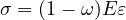
different directions decrease proportionally and independently of the loading direction. The damaged stiffness tensor is
expressed as D = (1 - ω)De where ω is a scalar damage variable and De is the elastic stiffness tensor. The damage
evolution law is postulated in an explicit form, relating the damage variable ω to the largest previously reached
equivalent strain level, κ.
The equivalent strain,  , is a scalar measure derived from the strain tensor. The choice of the specific expression for
the equivalent strain affects the shape of the elastic domain in the strain space and plays a similar role to the choice of
a yield condition in plasticity. The following definitions of equivalent strain are currently supported:
, is a scalar measure derived from the strain tensor. The choice of the specific expression for
the equivalent strain affects the shape of the elastic domain in the strain space and plays a similar role to the choice of
a yield condition in plasticity. The following definitions of equivalent strain are currently supported:
-
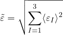
Mazars (1984) definition based on norm of positive part of strain:
where ⟨εI⟩ are positive parts of principal values of the strain tensor ε.
-
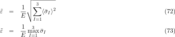
Definitions derived from the Rankine criterion of maximum principal stress:
where σI, I = 1,2,3, are the principal values of the effective stress tensor σ = De : ε and ⟨σI⟩ are their positive
parts.
-
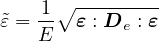
Energy norm scaled by Young’s modulus to obtain a strain-like quantity:
-
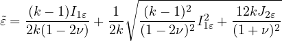
Modified Mises definition, proposed by de Vree [27]:
where
is the first strain invariant (trace of the strain tensor),
is the second deviatoric strain invariant, and k is a model parameter that corresponds to the ratio between the
uniaxial compressive strength fc and uniaxial tensile strength ft.
-
Griffith definition with a solution on inclined elipsoidal inclusion. This definition handles materials in pure
tension and also in compression, where tensile stresses usually appear on specifically oriented elipsoidal inclusion.
The derivation of Griffith’s criterion is summarized in [15]. In impementation, first check if Rankine criterion
applies
and if not, use Griffith’s solution with ordered principal stresses σ1 > σ3. The optional parameter griff_n is by
default 8 and represents the uniaxial compression/tensile strength ratio.
Note that all these definitions are based on the three-dimensional description of strain (and stress). If they are used
in a reduced problem, the strain components that are not explicitly provided by the finite element approximation are
computed from the underlying assumptions and used in the evaluation of equivalent strain. For instance, in a
plane-stress analysis, the out-of-plane component of normal strain is calculated from the assumption of zero
out-of-plane normal stress (using standard Hooke’s law).
Since the growth of damage usually leads to softening and may induce localization of the dissipative process,
attention should be paid to proper regularization. The most efficient approach is based on a nonlocal formulation; see
Section 1.5.7. If the model is kept local, the damage law should be adjusted according to the element size, in the spirit
of the crack-band approach. When done properly, this ensures a correct dissipation of energy in a localized band of
cracking elements, corresponding to the fracture energy of the material. For various numerical studies, it may be useful
to specify the parameters of the damage law directly, independently of the element size. One should be aware that in
this case the model would exhibit pathological sensitivity to the size of finite elements if the mesh is
changed.
The following damage laws are currently implemented:
-
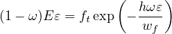
Cohesive crack with exponential softening postulates a relation between the normal stress σ
transmitted by the crack and the crack opening w in the form
Here, ft is the tensile strength and wf is a parameter with the dimension of length (crack opening),
which controls the ductility of the material. In fact, wf = Gf∕ft where Gf is the mode-I fracture energy.
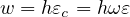
In the context of the crack-band approach, the crack opening w corresponds to the inelastic (cracking)
strain εc multiplied by the effective thickness h of the crack band. The effective thickness h is estimated
by projecting the finite element onto the direction of the maximum principal strain (and stress) at the
onset of damage. The inelastic strain εc is the difference between the total strain ε and the elastic strain
σ∕E. For the damage model we obtain
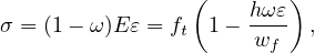
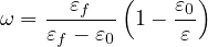
and thus w = hεc = hωε. Substituting this into the cohesive law and combining with the stress-strain
law for the damage model, we get a nonlinear equation
For a given strain ε, the corresponding damage variable ω can be solved from this equation by Newton
iterations. It can be shown that the solution exists and is unique for every ε ≥ ε0 provided that the
element size h does not exceed the limit size hmax = wf∕ε0. For larger elements, a local snapback in the
stress-strain diagram would occur, which is not admissible. In terms of the material properties, hmax can
be expressed as EGf∕ft2, which is related to Irwin’s characteristic length.
The derivation has been performed for monotonic loading and uniaxial tension. Under general conditions,
ε is replaced by the internal variable κ, which represents the maximum previously reached level of
equivalent strain.
In the list of input variables, the tensile strength ft is not specified directly but through the corresponding
strain at peak stress, ε0 = ft∕E, denoted by keyword e0. Another input parameter is the characteristic
crack opening wf, denoted by keyword wf.
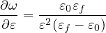
Derivative can be expressed explicitly
-
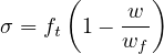
Cohesive crack with linear softening is based on the same correspondence between crack opening
and inelastic strain, but the cohesive law is assumed to have a simpler linear form
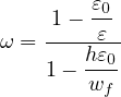
The relation between damage and strain can then be derived from the cohesive law and substituing
w = hωε
which leads to explicit evaluation of the damage variable
and no iteration is needed. Parameter wf, denoted again by keyword wf, has now the meaning of crack
opening at complete failure (zero cohesive stress) and is related to fracture energy by a modified formula
wf = 2Gf∕ft. The expression for maximum element size, hmax = wf∕ε0, remains the same as for
cohesive law with exponential softening, but in terms of the material properties it is now translated as
hmax = 2EGf∕ft2. The derivative with respect to ε yields
-
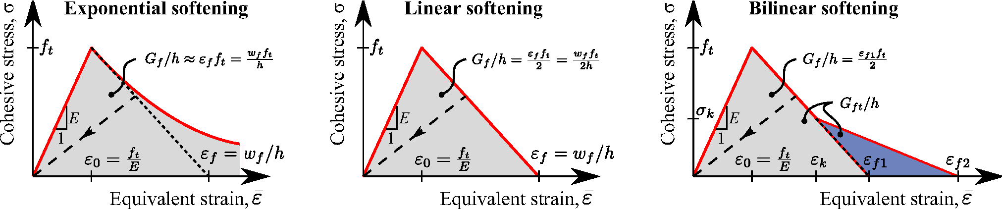
Cohesive crack with bilinear softening is implemented in an approximate fashion and gives for
different mesh sizes the same total dissipation but different shapes of the softening diagram. Instead
of properly transforming the crack opening into inelastic strain, the current implementation deals with
a stress-strain diagram adjusted such that the areas marked in the right part of Fig. 7 are equal to
the fracture energies Gf and Gft divided by the element size. The third parameter defining the law
is the strain εk at which the softening diagram changes slope. Since this strain is considered as fixed,
the corresponding stress σk depends on the element size and for small elements gets close to the tensile
strength (the diagram then gets close to linear softening with fracture energy Gft).
-
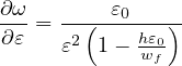
Linear softening stress-strain law works directly with strain and does not make any adjustment for
the element size. The specified parameters ε0 and εf, denoted by keywords e0 and ef, have the meaning
of (equivalent) strain at peak stress and at complete failure. The linear relation between stress and strain
on the softening branch is obtained with the damage law
Again, to cover general conditions, ε is replaced by κ.
-
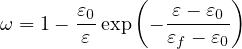
Exponential softening stress-strain law also uses two parameters ε0 and εf, denoted by keywords
e0 and ef, but leads to a modified dependence of damage on strain:
-
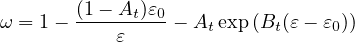
Mazars stress-strain law uses three parameters, ε0, At and Bt, denoted by keywords e0, At and Bt,
and the dependence of damage on strain is given by
-
Smooth exponential stress-strain law uses two parameters, ε0 and Md, denoted by keywords e0
and md, and the dependence of damage on strain is given by
This leads to a stress-strain curve that immediately deviates from linearity (has no elastic part) and
smoothly changes from hardening to softening, with tensile strength
-
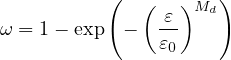
Extended smooth stress-strain law is a special formulation used by Grassl and Jirásek [10]. The damage law
has a rather complicated form:
The primary model parameters are the uniaxial tensile strength ft, the strain at peak stress (under uniaxial
tension) εp, and additional parameters ε1, ε2 and n, which control the post-peak part of the stress-strain law. In
the input record, they are denoted by keywords ft, ep, e1, e2, nd. Other parameters that appear in (78) can be
derived from the condition of zero slope of the stress-strain curve at κ = εp and from the conditions of stress and
stiffness continuity at κ = ε1:
-
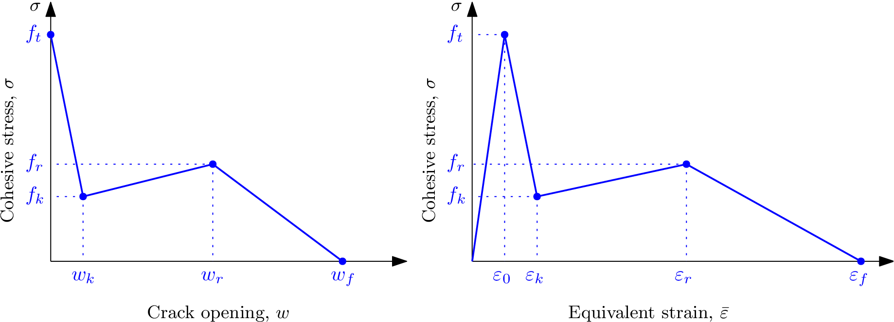
Trilinear softening is a special formulation proposed by Prof. Gálvez’s group to cope with fibre reinforced
concrete fracture [11]. It is formulated for an embedded crack model and it is expressed in terms of
crack opening (w). This approach uses a trilinear softening diagram that helps reproducing the
FRC behaviour; this diagram is defined by four points: t, k, r and f that are related to specific
properties of concrete, fibres and the fibre proportion. In order to adapt the original formulation to
the idm1, which uses damage ω as the driving parameter of fracture, instead of crack opening
w, the correspondence between both must be taken into account. Figure 6 shows the trilinear
diagram expressed in terms of the crack opening w (left) and in terms of the equivalent strain ε
(right).
The inelastic strain εc is the difference between the total strain ε and the elastic strain ε∕E, thus:
If σ is obtained by using the damage parameter (ω) , it can be expressed as follows:
Therefore, the inelastic strain can be written as:
Thus, crack opening (w) is related to damage (ω)
through :
where h stands for the effective thickness of the crack band, which is estimated by projecting the finite elmeent
onto the direction of the maximum principal strain at the onset of damage.
Hereafter, the expressions of damage (ω) are obtained for each section of the softening diagram (before damage
develops, damage between points t and k, between points k and r, between points r and f and, finally, after
damage has fully developed).
-
Case 1: ε ≤ ε0 : In this case, damage has not started, thus:
And its derivative:
-
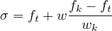
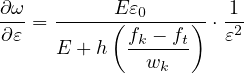
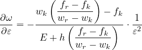
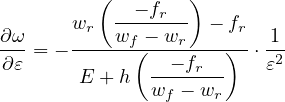
Case 2: ε0 ≤ ε ≤ εk : Referred to the σ - w diagram:
therefore, since ft = Eε0 and using expressions (82) and (83):
ω = 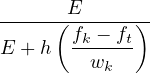 - -![-------E-ε0--------
[ ( fk --ft)]
ε E + h wk](matlibmanual100x.png) | | |
And its derivative:
-
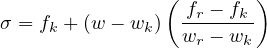
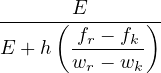
Case 3: εk ≤ ε ≤ εr : Referred to the σ - w diagram:
therefore, using expressions (82) and (83):
And its derivative:
-
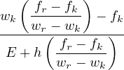
Case 4: εr ≤ ε ≤ εf : Referred to the σ - w diagram:
therefore, using expressions (82) and (83):
And its derivative:
-
Case 5: ε ≥ εf : In this case, damage is fully developed:
Note that parameter damlaw determines which type of damage law should be used, but the adjustment for element
size is done only if parameter wf is specified for damlaw=0 or damlaw=1. For other values of damlaw, or if parameter
ef is specified instead of wf, the stress-strain curve does not depend on element size and the model would
exhibit pathological sensitivity to the mesh size. These cases are intended to be used in combination
with a nonlocal formulation. An alternative formulation uses fracture energy to determine fracturing
strain.
The model parameters are summarized in Tab. 26. Figure 7 shows three modes of a softening law with
corresponding variables.
|
|
| Description |
Isotropic damage model for concrete in tension |
|
|
| Record Format |
Idm1 (in) # d(rn) # E(rn) # n(rn) # [tAlpha(rn) #]
[equivstraintype(in) #] [k(rn) #] [damlaw(in) #]
e0(rn) # [wf(rn) #] [ef(rn) #] [ek(rn) #] [wk(rn) #] [sk(rn) #]
[wkwf(rn) #] [skft(rn) #] [gf(rn) #] [gft(rn) #] [At(rn) #]
[Bt(rn) #] [md(rn) #] [ft(rn) #]
[ep(rn) #] [e1(rn) #] [e2(rn) #] [nd(rn) #] [maxOmega(rn) #]
[checkSnapBack(rn) #] |
| Parameters |
- material number |
| |
- d material density |
| |
- E Young’s modulus |
| |
- n Poisson’s ratio |
| |
- tAlpha thermal expansion coefficient |
| |
- equivstraintype allows to choose from different definitions of
equivalent strain:
-
default = Mazars, eq. (71)
-
smooth Rankine, eq. (72)
-
scaled energy norm, eq. (74)
-
modified Mises, eq. (75)
-
standard Rankine, eq. (73)
-
elastic energy based on positive stress
-
elastic energy based on positive strain
-
Griffith criterion eq. (77)
|
| |
- k ratio between uniaxial compressive and tensile strength,
needed only if equivstraintype=3, default value 1 |
| |
- damlaw allows to choose from different damage laws:
-
exponential softening (default) with parameters e0
and wf | ef | gf
-
linear softening with parameters e0 and wf | ef | gf
-
bilinear softening with (e0, gf, gft, ek) | (e0, wk, sk,
wf) | (e0, wkwf, skft, wf) | (e0, gf, gft, wk)
-
Hordijk softening (not implemented yet)
-
Mazars damage law with parameters At and Bt
-
smooth stress-strain curve with parameters e0 and md
-
disable damage (dummy linear elastic material)
-
extended smooth damage law (78) with parameters
ft, ep, e1, e2, nd
-
trilinear softening diagram with (e0, w_k, w_r, w_f,
f_k, f_r)
|
| |
- e0 strain at peak stress (for damage laws 0,1,2,3), limit
elastic strain (for damage law 4), characteristic strain (for
damage law 5) |
| |
- wf parameter controling ductility, has the meaning of crack
opening (for damage laws 0 and 1) |
| |
- ef parameter controling ductility, has the meaning of strain
(for damage laws 0 and 1) |
| |
- ek strain at knee point in bilinear softening type (for
damage law 2) |
| |
- wk crack opening at knee point in bilinear softening type
(for damage law 2) |
| |
- sk stress at knee point in bilinear softening type (for
damage law 2) |
| |
- wkwf ratio of wk/wf < 0,1 > in bilinear softening type
(for damage law 2) |
| |
- skft ratio of sk/ft < 0,1 > in bilinear softening type (for
damage law 2) |
| |
- gf fracture energy (for damage laws 0–2) |
| |
- gft total fracture energy (for damage law 2) |
| |
- At parameter of Mazars damage law, used only by law 4 |
| |
- Bt parameter of Mazars damage law, used only by law 4 |
| |
- md exponent used only by damage law 5, default value 1 |
| |
- ft tensile strength, used only by damage law 7 |
| |
- ep strain at peak stress, used only by damage law 7 |
| |
- e1 parameter used only by damage law 7 |
| |
- e2 parameter used only by damage law 7 |
| |
- nd exponent used only by damage law 7 |
| |
- griff_n uniaxial compression/tensile ratio for Griffith’s
criterion |
| |
- maxOmega maximum damage, used for convergence
improvement (its value is between 0 and 0.999999 (default),
and it affects only the secant stiffness but not the stress) |
| |
- checkSnapBack parameter for snap back checking, 0 no
check, 1 check (default) |
| |
- w_k crack opening of point k in the trilinear diagram (see
Fig. 6) |
| |
- w_r crack opening of point r in the trilinear diagram (see
Fig. 6) |
| |
- w_f crack opening of point f in the trilinear diagram (see
Fig. 6) |
| |
- f_k cohesive stress of point k in the trilinear diagram (see
Fig. 6) |
| |
- f_r cohesive stress of point r in the trilinear diagram (see
Fig. 6) |
| Supported modes |
3dMat, PlaneStress, PlaneStrain, 1dMat |
| Features |
Adaptivity support |
|
|
| Table 26: Isotropic damage model for tensile failure – summary. |
| |
| |
| |
| | |
1.5.7 Nonlocal isotropic damage model for tensile failure - Idmnl1
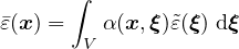
Nonlocal version of isotropic damage model from Section 1.5.6. The nonlocal averaging acts as a powerful localization
limiter. In the standard version of the model, damage is driven by the nonlocal equivalent strain ε, defined as a
weighted average of the local equivalent strain:
In the “undernonlocal” formulation, the damage-driving variable is a combination of local and nonlocal equivalent
strain, mε + (1 -m) , where m is a parameter between 0 and 1. (If m > 1, the formulation is called “overnonlocal”;
this case is useful for nonlocal plasticity but not for nonlocal damage.)
, where m is a parameter between 0 and 1. (If m > 1, the formulation is called “overnonlocal”;
this case is useful for nonlocal plasticity but not for nonlocal damage.)
Instead of averaging the equivalent strain, one can average the compliance variable γ, directly related to damage
according to the formula γ = ω∕(1 - ω).
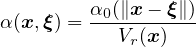
The weight function α contains a certain parameter with the dimension of length, which is in general called the
characteristic length. Its specific meaning depends on the type of weight function. The following functions are
currently supported:
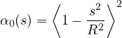
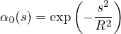
-
Truncated quartic spline, also called the bell-shaped function,
where R is the interaction radius (characteristic length) and s is the distance between the interacting
points. This function is exactly zero for s ≥ R, i.e., it has a bounded support.
-
Gaussian function
which is theoretically nonzero for an arbitrary large s and thus has an unbounded support. However, in
the numerical implementation the value of α0 is considered as zero for s > 2.5R.
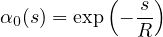
-
Exponential function
which also has an unbounded support, but is considered as zero for s > 6R. This function is sometimes
called the Green function, because in 1D it corresponds to the Green function of the Helmholtz-like
equation used by implicit gradient approaches.
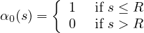
-
Piecewise constant function
which corresponds to uniform averaging over a segment, disc or ball of radius R.
-
Function that is constant over the finite element in which point x is located, and is zero everywhere
else. Of course, this is not a physically objective definition of nonlocal averaging, since it depends on the
discretization. However, this kind of averaging was proposed in a boundary layer by Prof. Bažant and
was implemented into OOFEM for testing purposes.
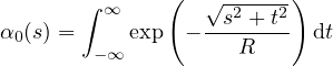
-
Special function
obtained by reduction of the exponential function from 2D to 1D. The integral cannot be evaluated in
closed form and is computed by OOFEM numerically. This function can be used in one-dimensional
simulations of a two-dimensional specimen under uniaxial tension; for more details see [12].
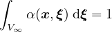
The above functions depend only on the distance s between the interacting points and are not normalized. If the
normalizing condition
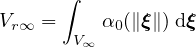
is imposed in an infinite body V ∞, it is sufficient to scale α0 by a constant and set
where
Constant V r∞ can be computed analytically depending on the specific type of weight function and the number of
spatial dimensions in which the analysis is performed. Since the factor 1∕V r∞ can be incorporated directly in the
definition of α0, this case is referred to as “no scaling”.
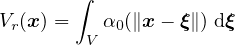
If the body of interest is finite (or even semi-infinite), the averaging integral can be performed only over the
domain filled by the body, and the volume contributing to the nonlocal average at a point x near the boundary is
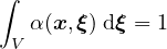
reduced as compared to points x far from the boundary or in an infinite body. To make sure that the normalizing
condition
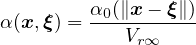
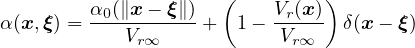
holds for the specific domain V , different approaches can be used. The standard approach defines the nonlocal
weight function as
where
According to the approach suggested by Borino, the weight function is defined as
where δ is the Dirac distribution. One can also say that the nonlocal variable is evaluated as
The term on the right-hand side after the integral is a multiple of the local variable, and so it can be referred to as
the local complement.
In a recent paper [12], special techniques that modify the averaging procedure based on the distance
from a physical boundary of the domain or on the stress state have been considered. The details are
explained in [12]. These techniques can be invoked by setting the optional parameter nlVariation to 1, 2
or 3 and specifying additional parameters β and ζ for distance-based averaging, or β for stress-based
averaging.
The model parameters are summarized in Tabs. 27 and 28.
|
|
| Description | Nonlocal isotropic damage model for concrete in tension |
|
|
|
Record Format | Idmnl1 (in) # d(rn) # E(rn) # n(rn) # [tAlpha(rn) #]
[equivstraintype(in) #] [k(rn) #] [damlaw(in) #] e0(rn) #
[ef(rn) #] [At(rn) #] [Bt(rn) #] [md(rn) #]
r(rn) # [regionMap(ia) #] [wft(in) #] [averagingType(in) #]
[m(rn) #] [scalingType(in) #]
[averagedQuantity(in) #] [nlVariation(in) #] [beta(rn) #]
[zeta(rn) #] [maxOmega(rn) #]
|
| Parameters | - material number |
|
| - d material density |
|
| - E Young’s modulus |
| | - n Poisson’s ratio |
| | - tAlpha thermal expansion coefficient |
|
| - equivstraintype allows to choose from different definitions
of equivalent strain, same as for the local model; see
Tab. 26
|
|
| - k ratio between uniaxial compressive and tensile strength,
needed only if equivstraintype=3, default value 1
|
|
| - damlaw allows to choose from different damage laws, same
as for the local model; see Tab. 26 (note that parameter wf
cannot be used for the nonlocal model)
|
|
| - e0 strain at peak stress (for damage laws 0,1,2,3), limit
elastic strain (for damage law 4), characteristic strain (for
damage law 5)
|
|
| - ef strain parameter controling ductility, has the meaning
of strain (for damage laws 0 and 1), the tangent modulus
just after the peak is Et = -ft∕(εf - ε0)
|
| | - At parameter of Mazars damage law, used only by law 4 |
| | - Bt parameter of Mazars damage law, used only by law 4 |
| | - md exponent, used only by damage law 5, default value 1 |
|
| - r nonlocal characteristic length R; its meaning depends
on the type of weight function (e.g., interaction radius for
the quartic spline)
|
|
| - regionMap map indicating the regions (currently region
is characterized by cross section number) to skip for
nonlocal avaraging. The elements and corresponding IP are
not taken into account in nonlocal averaging process if
corresponding regionMap value is nonzero.
|
|
| - wft selects the type of nonlocal weight function:
-
default, quartic spline (bell-shaped function with
bounded support)
-
Gaussian function
-
exponential function (Green function in 1D)
-
uniform averaging up to distance R
-
uniform averaging over one finite element
-
special function obtained by reducing the 2D
exponential function to 1D (by numerical integration)
|
| | — continued in Tab. 28 — |
|
|
| |
Table 27: Nonlocal isotropic damage model for tensile failure – summary.
|
|
| Description | Nonlocal isotropic damage model for concrete in tension |
|
|
|
| - averagingType activates a special averaging procedure,
default value 0 does not change anything, value 1 means
averaging over one finite element (equivalent to wft=5, but
kept here for compatibility with previous version)
|
|
| - m multiplier for overnonlocal
or undernonlocal formulation, which use m-times the local
variable plus (1 - m)-times the nonlocal variable, default
value 1
|
|
| - scalingType selects the type of scaling of the weight function
(e.g. near a boundary):
-
default, standard scaling with integral of weight
function in the denominator
-
no scaling (the weight function normalized in an
infinite body is used even near a boundary)
-
Borino scaling (local complement)
|
|
| - averagedQuantity selects the variable to be averaged,
default value 1 corresponds to equivalent strain, value 2
activates averaging of compliance variable
|
|
| - nlVariation activates a special averaging procedure,
default value 0 does not change anything, value 1 means
distance-based averaging (the characteristic length is
linearly reduced near a physical boundary), value 2 means
stress-based averaging (the averaging is anisotropic and
the characteristic length is affected by the stress), value 3
means distance-based averaging (the characteristic length
is exponentially reduced near a physical boundary)
|
|
| - beta parameter β, required only for distance-based and
stress-based averaging (i.e., for nlVariation=1, 2 or 3)
|
|
| - zeta parameter ζ, required only for distance-based
averaging (i.e., for nlVariation=1 or 3)
|
|
| - maxOmega maximum damage, used for convergence
improvement (its value is between 0 and 0.999999 (default),
and it affects only the secant stiffness but not the stress)
|
| Supported modes | 3dMat, PlaneStress, PlaneStrain, 1dMat |
| Features | Adaptivity support |
|
|
| |
Table 28: Nonlocal isotropic damage model for tensile failure – continued.
1.5.8 Anisotropic damage model - Mdm
Local formulation
The concept of isotropic damage is appropriate for materials weakened by voids, but if the physical source of
damage is the initiation and propagation of microcracks, isotropic stiffness degradation can be considered
only as a first rough approximation. More refined damage models take into account the highly oriented
nature of cracking, which is reflected by the anisotropic character of the damaged stiffness or compliance
matrices.
A number of anisotropic damage formulations have been proposed in the literature. Here we use a model outlined
by Jirásek [17], which is based on the principle of energy equivalence and on the construction of the inverse integrity
tensor by integration of a scalar over all spatial directions. Since the model uses certain concepts from the microplane
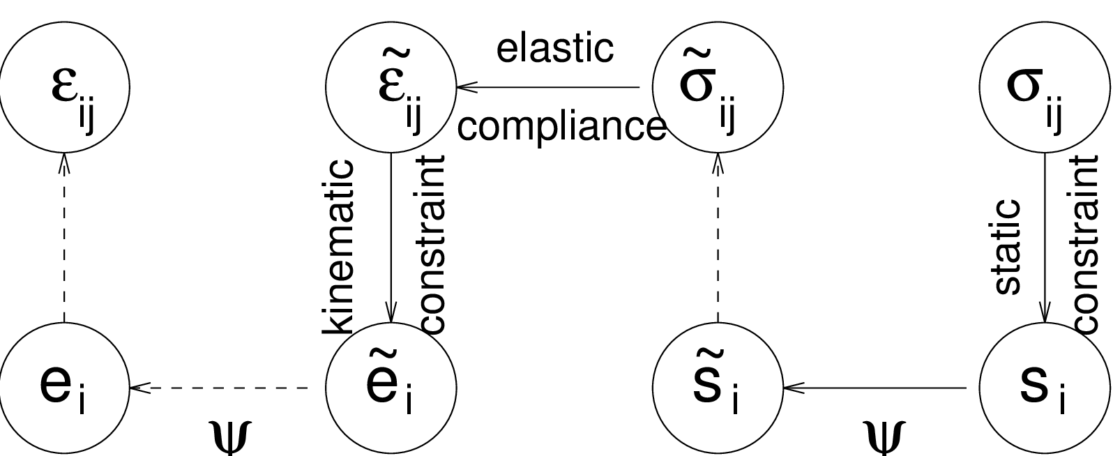
theory, it is called the microplane-based damage model (MDM).
The general structure of the MDM model is schematically shown in Fig. 8 and the basic equations are summarized
in Tab. 29. Here, ε and σ are the (nominal) second-order strain and stress tensors with components εij and σij; e and
s are first-order strain and stress tensors with components ei and si, which characterize the strain and
stress on “microplanes” of different orientations given by a unit vector n with components ni; ψ is a
dimensionless compliance parameter that is a scalar but can have different values for different directions
n; the symbol δ denotes a virtual quantity; and a sumperimposed tilde denotes an effective quantity,
which is supposed to characterize the state of the intact material between defects such as microcracks or
voids.
Table 29: Basic equations of microplane-based anisotropic damage model
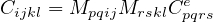
Combining the basic equations, it is possible to show that the components of the damaged material compliance
tensor are given by
where Cpqrse are the components of the elastic material compliance tensor,
are the components of the so-called damage effect tensor, and
are the components of the second-order inverse integrity tensor. The integration domain Ω is the unit hemisphere. In
practice, the integral over the unit hemisphere is evaluated by summing the contribution from a finite
number of directions, according to one of the numerical integration schemes that are used by microplane
models.
The scalar variable ψ characterizes the relative compliance in the direction given by the vector n. If ψ is the same
in all directions, the inverse integrity tensor evaluated from (86) is equal to the unit second-order tensor (Kronecker
delta) multiplied by ψ, the damage effect tensor evaluated from (85) is equal to the symmetric fourth-order unit tensor
multiplied by ψ, and the damaged material compliance tensor evaluated from (84) is the elastic compliance tensor
multiplied by ψ2. The factor multiplying the elastic compliance tensor in the isotropic damage model is
1∕(1 - ω), and so ψ corresponds to 1∕ . In the initial undamaged state, ψ = 1 in all directions. The
evolution of ψ is governed by the history of the projected strain components. In the simplest case, ψ is
driven by the normal strain eN = εijninj. Analogy with the isotropic damage model leads to the damage
law
. In the initial undamaged state, ψ = 1 in all directions. The
evolution of ψ is governed by the history of the projected strain components. In the simplest case, ψ is
driven by the normal strain eN = εijninj. Analogy with the isotropic damage model leads to the damage
law
and loading-unloading conditions
in which κ is a history variable that represents the maximum level of normal strain in the given direction ever reached
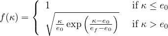
in the previous history of the material. An appropriate modification of the exponential softening law leads to the
damage law
where e0 is a parameter controlling the elastic limit, and ef > e0 is another parameter controlling ductility. Note that
softening in a limited number of directions does not necessarily lead to softening on the macroscopic level, because the
response in the other directions remains elastic. Therefore, e0 corresponds to the elastic limit but not to the state at
peak stress.
If the MDM model is used in its basic form described above, the compressive strength turns out to depend on the
Poisson ratio and, in applications to concrete, its value is too low compared to the tensile strength. The model is
designed primarily for tensile-dominated failure, so the low compressive strength is not considered as a major
drawback. Still, it is desirable to introduce a modification that would prevent spurious compressive failure in problems
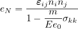
where moderate compressive stresses appear. The desired effect is achieved by redefining the projected strain eN
as
where m is a nonnegative parameter that controls the sensitivity to the mean stress, σkk is the trace of the stress
tensor, and the normalizing factor Ee0 is introduced in order to render the parameter m dimensionless. Under
compressive stress states (characterized by σkk < 0), the denominator in (90) is larger than 1, and the projected strain
is reduced, which also leads to a reduction of damage. A typical recommended value of parameter m is
0.05.
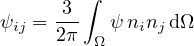
Nonlocal formulation
Nonlocal formulation of the MDM model is based on the averaging of the inverse integrity tensor. This roughly
corresponds to the nonlocal isotropic damage model with averaging of the compliance variable γ = ω∕(1 -ω), which
does not cause any spurious locking effects. In equation (85) for the evaluation of the damage effect tensor, the inverse
integrity tensor is replaced by its weighted average with components
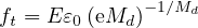
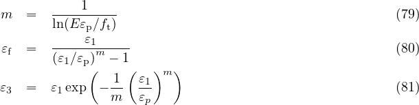
By fitting a wide range of numerical results, it has been found that the parameters of the nonlocal MDM model
can be estimated from the measurable material properties using the formulas
where E is Young’s modulus, Gf is the fracture energy, ft is the uniaxial tensile strength, m is the compressive
correction factor, typically chosen as m = 0.05, and R is the radius of nonlocal interaction reflecting the internal
length of the material.
Input Record
The model description and parameters are summarized in Tab. 30.
|
|
| Description | MDM Anisotropic damage model |
|
|
| | Common parameters |
|
Record Format | Mdm d(rn) # nmp(ins) # talpha(rn) # parmd(rn) #
nonloc(in) # formulation(in) # mode(in) #
|
| Parameters | -num material model number |
|
| - D material density |
|
| - nmp number of microplanes used for hemisphere
integration, supported values are 21,28, and 61
|
| | - talpha thermal dillatation coeff |
| | - parmd |
| | - nonloc |
|
| - formulation |
| | - mode |
|
|
| Nonlocal variant I | |
|
Additional params | r(rn) # efp(rn) # ep(rn) # |
| | -r nonlocal interaction radius |
|
| -efp εfp is a model parameter that controls the post-peak
slope εfp =εf - ε0, where εf is strain at zero stress level.
|
| | -ep max effective strain at peak ε0 |
|
|
| Nonlocal variant II | |
| Additional params | r(rn) # gf(rn) # ft(rn) # |
| | -r nonlocal intraction radius |
| | -gf fracture energy |
| | -ft tensile strength |
|
|
| Local variant I | |
| Additional params | efp(rn) # ep(rn) # |
|
| -efp εfp is a model parameter that controls the post-peak
slope εfp =εf - ε0, where εf is strain at zero stress level.
|
| | -ep max effective strain at peak ε0 |
|
|
| Local variant II | |
| Additional params | gf(rn) # ep(rn) # |
| | -gf fracture energy |
| | -ep max effective strain at peak ε0 |
|
|
| Supported modes | 3dMat, PlaneStress |
| Features | Adaptivity support |
|
|
| |
Table 30: MDM model - summary.
1.5.9 Isotropic damage model for interfaces
The model provides an interface law which can be used to describe a damageable interface between two materials
(e.g. between steel reinforcement and concrete). The law is formulated in terms of the traction vector and the
displacement jump vector. The basic response is elastic, with stiffness kn in the normal direction and ks in the
tangential direction. Similar to other isotropic damage models, this model assumes that the stiffness degradation is
isotropic, i.e., both stiffness moduli decrease proportionally and independently of the loading direction. The damaged
stiffnesses are kn×(1 -ω) and ks×(1 -ω) where ω is a scalar damage variable. The damage evolution law is postulated
in an explicit form, relating the damage variable ω to the largest previously reached equivalent “strain” level,
κ.
The equivalent “strain”,  , is a scalar measure of the displacement jump vector. The choice of the specific
expression for the equivalent strain affects the shape of the elastic domain in the strain space and plays a similar role
to the choice of a yield condition in plasticity. Currently, in the present implementation, the equivalent strain is given
by
, is a scalar measure of the displacement jump vector. The choice of the specific
expression for the equivalent strain affects the shape of the elastic domain in the strain space and plays a similar role
to the choice of a yield condition in plasticity. Currently, in the present implementation, the equivalent strain is given
by
where ⟨wn⟩ is the positive part of the normal displacement jump (opening of the interface) and ws is the norm of
the tangential part of displacement jump (sliding of the interface). Parameter β is optional and its default value is 0,
in which case damage depends on the opening only (not on the sliding). The dependence of damage ω on
maximum equivalent strain κ is described by the following damage law which corresponds to exponential
softening:
Here, ε0 = ft∕kn is the value of equivalent strain at the onset of damage. Note that if the interface is subjected to
shear traction only (with zero or negative normal traction), the propagation of damage starts when the magnitude
of the sliding displacement is |ws| = ε0∕ , i.e., when the magnitude of the shear traction is equal
to
, i.e., when the magnitude of the shear traction is equal
to
So the ratio between the shear strength and tensile strength of the interface, fs∕ft, is equal to ks∕kn .
.
The model parameters are summarized in Tab. 31.
|
|
| Description | Isotropic damage model for concrete in tension |
|
|
|
Record Format | isointrfdm01 kn(rn) # ks(rn) # ft(rn) # gf(rn) #
[ maxomega(rn) #] talpha(rn) # d(rn) #
|
| Parameters | - d material density |
| | - tAlpha thermal dilatation coefficient |
| | - kn elastic stifness in normal direction |
|
| - ks elastic stifness in tangential direction |
|
| - ft tensile strength |
|
| - gf fracture energy |
|
| - [maxomega] maximum damage, used for convergence
improvement (its value is between 0 and 0.999999 (default), and
it affects only the secant stiffness but not the stress)
|
|
| - [beta] parameter controlling the effect of sliding part of
displacement jump on equivalent strain, default value 0
|
| Supported modes | 2dInterface, 3dInterface |
| Features | |
|
|
| |
Table 31: Isotropic damage model for interface elements – summary.
1.5.10 Isotropic damage model for interfaces using tabulated data for damage
The model provides an interface law which can be used to describe a damageable interface between two materials
(e.g. between steel reinforcement and concrete). The law is formulated in terms of the traction vector and the
displacement jump vector. The basic response is elastic, with stiffness kn in the normal direction and ks in the
tangential direction. Similar to other isotropic damage models, this model assumes that the stiffness
degradation is isotropic, i.e., both stiffness moduli decrease proportionally and independently of the
loading direction. The damaged stiffnesses are kn×(1 - ω) and ks×(1 - ω) where ω is a scalar damage
variable.
The equivalent “strain”,  , is a scalar measure derived from the displacement jump vector. The choice of the
specific expression for the equivalent strain affects the shape of the elastic domain in the strain space and plays a
similar role to the choice of a yield condition in plasticity. Currently, in the present implementation,
, is a scalar measure derived from the displacement jump vector. The choice of the
specific expression for the equivalent strain affects the shape of the elastic domain in the strain space and plays a
similar role to the choice of a yield condition in plasticity. Currently, in the present implementation,  is equal to the
positive part of the normal displacement jump (opening of the interface).
is equal to the
positive part of the normal displacement jump (opening of the interface).
The damage evolution law is postulated in a separate file that should have the following format.
Each line should contain one strain, damage pair separated by a whitespace character. The exception to
this is the first line which should contain a single integer stating how many strain, damage pairs that
the file will contain. The strains given in the file is defined as the equivalent strain minus the limit of
elastic deformation. To find the damage for arbitrary strains linear interpolation between the tabulated
values is used. If a strain larger than one in the given table is achieved the respective damage for the
largest tabulated strain will be used. Both the strains and damages must be given in a strictly increasing
order.
The model parameters are summarized in Tab. 32.
|
|
| Description | Isotropic damage model for concrete in tension |
|
|
|
Record Format | isointrfdm02 kn(rn) # ks(rn) # ft(rn) # tablename(rn) #
[ maxomega(rn) #] talpha(rn) # d(rn) #
|
| Parameters | - d material density |
| | - tAlpha thermal dilatation coefficient |
| | - kn elastic stifness in normal direction |
|
| - ks elastic stifness in tangential direction |
|
| - ft tensile strength |
| | - tablename file name of the table with the strain damage pairs |
|
| - maxomega maximum damage, used for convergence
improvement (its value is between 0 and 0.999999 (default), and
it affects only the secant stiffness but not the stress)
|
| Supported modes | 2dInterface, 3dInterface |
| Features | |
|
|
| |
Table 32: Isotropic damage model for interface elements using tabulated data for damage – summary.


![[ ] ( )
∂ω-= ----1----+ -1 ε0 exp -ε0 --ε
∂ε ε(εf - ε0) ε2 εf - ε0](matlibmanual86x.png)
![( ( ( )m ) )
||| 1 - exp - 1- ε- if ε ≤ ε1 |||
|{ (m εp ) |}
ω = | ε3 ε - ε1 |
|||( 1 - ε-exp( - --[---(ε-ε1)n]) if ε > ε1 |||)
εf 1+ -ε2-](matlibmanual90x.png)


 +
+ 
 +
+ 


 =
= 
 :
:  =
= 
 dΩ
dΩ 

 =
= 


![λ = EGf-- (92)
f Rft2
-----λf-------
λ = 1.47 - 0.0014λf (93)
f
e0 = ----------t---------- (94)
(1 - m)E (1.56+ 0.006λ )
ef = e0[1+ (1- m )λ ] (95)](matlibmanual149x.png)