Plasticity-based material models

1.4 Plasticity-based material models

1.4.1 Drucker-Prager model - DruckerPrager

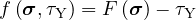
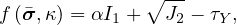
The Drucker-Prager plasticity model¹ is an isotropic elasto-plastic model based on a yield function

f (σ,τY) = F (σ )- τY

(21)

with the pressure-dependent equivalent stress

∘ -- F (σ) = αI1 + J2

(22)

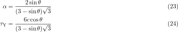
As usual, σ is the stress tensor, τY is the yield stress under pure shear, and I₁ and J₂ are the first invariant and second deviatoric invariant of the stress tensor. The friction coefficient α is a positive parameter that controls the influence of the pressure on the yield limit, important for cohesive-frictional materials such as concrete, soils or other geomaterials. Regarding Mohr-Coulomb plasticity, relation to cohesion, c, and the angle of friction, θ, exists for the Drucker-Prager model

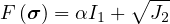
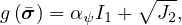
α = ---2-sinθ-√- (23) (3- sinθ) 3 6ccosθ τY = (3--sinθ)√3 (24)

The flow rule is derived from the plastic potential

∘ -- g(σ) = αψI1 + J2

(25)

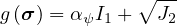
where αψ is the dilatancy coefficient. An associated model with αψ = α would overestimate the dilatancy of concrete, so the dilatancy coefficient is usually chosen smaller than the friction coefficient. The model is described by the equations

σ = D : (ε- ε ) (26) p τY = h(κ( ) ) (27) ˙ε = λ˙∂g- = ˙λ α δ+ -√s-- (28) p ∂σ ψ 2 J2 ∘ 2- κ˙ = -∥ε˙p∥ (29) 3

˙λ ≥ 0, f (σ, τY ) ≤ 0, λ˙f (σ,τY) = 0

(30)

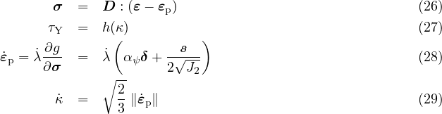
which represent the linear elastic law, hardening law, evolution laws for plastic strain and hardening variable, and the loading-unloading conditions. In the above, D is the elastic stiffness tensor, ε is the strain tensor, εp is the plastic strain tensor, λ is the plastic multiplier, δ is the unit second-order tensor, s is the deviatoric stress tensor, κ is the hardening variable, and a superior dot marks the derivative with respect to time. The flow rule has the form given in Eq. (28) at all points of the conical yield surface with the exception of its vertex, located on the hydrostatic axis.

For the present model, the evolution of the hardening variable can be explicitly linked to the plastic multiplier. Substituting the flow rule (28) into Eq. (29) and computing the norm leads to

κ˙= k˙λ

(31)

with a constant parameter k = ∘ --------2
1∕3 + 2αψ , so the hardening variable is proportional to the plastic multiplier. For α = αψ = 0, the associated J₂-plasticity model is recovered as a special case.

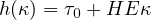
In the simplest case of linear hardening, the hardening function is a linear function of κ, given by

h(κ) = τ0 + HE κ

(32)

where τ₀ is the initial yield stress, and H is the hardening modulus normalized with the elastic modulus. Alternatively, an exponential hardening function

h(κ) = τlimit + (τ0 - τlimit)e-κ∕κc

(33)

can be used for a more realistic description of hardening.

The stress-return algorithm is based on the Newton-iteration. In plasticity, this is commonly called Closest-Point-Projection (CPP), and it generally leads to quadratic convergence. The implemented algorithm is convergent in any stress case, but in the vicinity of the vertex region, quadratic convergence might be lost because of insufficient regularity of the yield function.

The algorithmic tangent stiffness matrix is implemented for both the regular case and the vertex region. Generally, the error decreases quadratically (of course only asymptotically). Again, in the vicinity of the vertex region, quadratic convergence might be lost due to insufficient regularity. Furthermore, the tangent stiffness matrix does not always exist for the vertex case. In these cases, the elastic stiffness is used instead. It is generally safer (but slower) to use the elastic stiffness if you encounter any convergence problems, especially if your problem is tension-dominated.


Description	DP material

Record Format	DruckerPrager num(in) # d(rn) # tAlpha(rn) # E(rn) # n(rn) # alpha(rn) # alphaPsi(rn) # ht(in) # iys(rn) # lys(rn) # hm(rn) # kc(rn) # [ yieldtol(rn) #]
Parameters	- num material model number
	- d material density
	- tAlpha thermal dilatation coefficient
	- E Young modulus
	- n Poisson ratio
	- alpha friction coefficient
	- alphaPsi dilatancy coefficient
	- ht hardening type, 1: linear hardening, 2: exponential hardening
	- iys initial yield stress in shear, τ₀
	- lys limit yield stress for exponential hardening, τ_limit
	- hm hardening modulus normalized with E-modulus (!)
	- kc κ_c for the exponential softening law
	- yieldtol tolerance of the error in the yield criterion, default value 1.e-14
	- newtonIter maximum number of iterations in λ search, default value 30
Supported modes	3dMat, PlaneStrain, 3dRotContinuum

Table 11: DP material - summary.

1.4.2 Drucker-Prager model with tension cut-off and isotropic damage - DruckerPragerCut

The Drucker-Prager plasticity model with tension cut-off is a multisurface model, appropriate for cohesive-frictional materials such as concrete loaded both in compression and tension. The plasticity model is formulated for isotropic hardening and enhanced by isotropic damage, which is driven by the cumulative plastic strain. The model can be used only in the small-strain context, with additive split of the strain tensor into the elastic and plastic parts.

The basic equations include the additive decomposition of strain into elastic and plastic parts,

ε = εe + εp,

(34)

the stress strain law

σ = (1- ω)¯σ = (1- ω)D : (ε- εp),

(35)

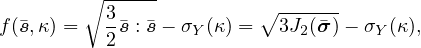
the definition of the yield function in terms of the effective stress,

∘ -- f (¯σ,κ) = αI1 + J2 - τY,

(36)

the flow rule

∘ -- g(¯σ) = α ψI1 + J2,

(37)

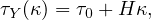
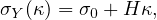
the linear hardening law

τY(κ) = τ0 + H κ,

(38)

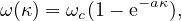
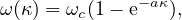
where τ₀ represents the initial yield stress under pure shear, the damage law

ω(κ) = ωc(1- e-aκ),

(39)

where ω_c is critical damage and a is a positive dimensionless parameter. More detailed descriptioin of some parameters is in Section 1.4.1.

The dilatancy coefficient αψ controls flow associativeness; if αψ = α, an associate model is recovered, which overestimates the dilatancy of concrete. Hence, the dilatancy coefficient is usually chosen smaller, αψ ≤ α, and the non-associated model is formulated.


Description	Drucker Prager material with tension cut-off

Record Format	DruckerPragerCut num(in) # d(rn) # tAlpha(rn) # E(rn) # n(rn) # tau0(rn) # alpha(rn) # [alphaPsi(rn) #] [H(rn) #] [omega_crit(rn) #] [a(rn) #] [yieldtol(rn) #] [NewtonIter(in) #]
Parameters	- num material model number
	- d material density
	- tAlpha thermal dilatation coefficient
	- E Young modulus
	- n Poisson ratio
	- tau0 initial yield stress in shear τ₀
	- alpha friction coefficient
	- alphaPsi dilatancy coefficient, equals to alpha by default
	- H hardening modulus (can be negative in the case of plastic softening), 0 by default
	- omega_crit critical damage in damage law (39), 0 by default
	- a exponent in damage law (39), 0 by default
	- yieldtol tolerance of the error in the yield criterion, default value 1.e-14
	- newtonIter maximum number of iterations in λ search, default value 30
Supported modes	1dMat, 3dMat, PlaneStrain

Table 12: Drucker Prager material with tension cut-off - summary.

1.4.3 Mises plasticity model with isotropic damage - MisesMat

This model is appropriate for the description of plastic yielding in ductile material such as metals, and it can also cover the effects of void growth. The model uses the Mises yield condition (in terms of the second deviatoric invariant, J₂), associated flow rule, linear isotropic hardening driven by the cumulative plastic strain, and isotropic damage, also driven by the cumulative plastic strain. The model can be used in the small-strain context, with additive split of the strain tensor into the elastic and plastic parts, or in the large-strain context, with multiplicative split of the deformation gradient and with yield condition formulated in terms of Kirchhoff stress (which is the true Cauchy stress multiplied by the Jacobian).

Small-strain formulation: The small-strain version of hardening Mises plasticity can be combined with isotropic damage. The basic equations include the additive decomposition of strain into elastic and plastic parts,

ε = εe + εp,

(40)

the stress strain law

σ = (1- ω)¯σ = (1- ω)D : (ε- εp),

(41)

the definition of the yield function in terms of the effective stress,

∘ ------ f(¯s,κ) = 3 ¯s : ¯s - σY (κ) = ∘3J2-(¯σ)- σY(κ), 2

(42)

the incremental definition of cumulative plastic strain

κ˙= ∥˙ε ∥, p

(43)

the linear hardening law (for htype = 0)

σ (κ) = σ + Hκ, Y 0

(44)

the evolution law for the plastic strain

∂f ˙εp = λ˙∂¯s,

(45)

the loading-unloading conditions

λ˙> 0 f(¯s,κ ) ≤ 0 ˙λf(¯s,κ ) = 0.

(46)

and the damage law

ω(κ) = ω (1- e-aκ), c

(47)

In the equations above, ε is the strain tensor, ε_e is the elastic strain tensor, ε_p is the plastic strain tensor, D is the elastic stiffness tensor, σ is the nominal stress tensor, σ is the effective stress tensor, s is the effective deviatoric stress tensor, σ_Y is the magnitude of stress at yielding under uniaxial tension (or compression), κ is the cumulated plastic strain, H is the hardening modulus, λ is the plastic multiplier, ω is the damage variable, ω_c is critical damage and a is a positive dimensionless parameter.

Large-strain formulation is based on the introduction of an intermediate local configuration, with respect to which the elastic response is characterized. This concept leads to a multiplicative decomposition of deformation gradient into elastic and plastic parts:

e p F = F F .

(48)

The stress-evaluation algorithm can be based on the classical radial return mapping; see [21] for more details. Damage is not yet implemented in the large-strain version of the model.

The model description and parameters are summarized in Tab. 13.


Description	Mises plasticity model with isotropic hardening

Record Format	MisesMat (in) # d(rn) # E(rn) # n(rn) # sig0(rn) # H(rn) # [ htype(in) #] [ h_eps(ra) #] [ h(eps)(ra) #] omega_crit(rn) #a(rn) #
Parameters	- material number
	- d material density
	- E Young’s modulus
	- n Poisson’s ratio
	- sig0 initial yield stress in uniaxial tension (compression) (Required if htype = 0, which is default)
	- H hardening modulus (can be negative in the case of plastic softening) (Required if htype = 0, which is default)
	- htype hardening type (Optional parameter. Default = 0)
	- h_eps array of plastic strains (Required if htype = 1)
	- h(eps) array of yield stresses (Required if htype = 1)
	- omega_crit critical damage in damage law (47)
	- a exponent in damage law (47)
Supported modes	1dMat, PlaneStrain, 3dMat, 3dMatF

Table 13: Mises plasticity – summary.

VTKxml output can report Mises stress, which equals to √ ---
3J2 . When no hardening/softening exists, Mises stress reaches values up to given uniaxial yield stress sig0.

1.4.4 Mises plasticity model with isotropic damage, nonlocal - MisesMatNl, MisesMatGrad

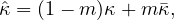
The small-strain version of the model is regularized by the over-nonlocal formulation with damage driven by a combination of local and nonlocal cumulated plastic strain,

ˆκ = (1 - m)κ+ m ¯κ,

(49)

where m is a dimensionless material parameter (typically m > 1) and κ is the nonlocal cumulated plastic strain, which is evaluated either using the integral approach, or using the implicit gradient approach.

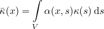
Integral nonlocal formulation One possible regularization technique is based on the integral definition of nonlocal cumulated plastic strain

∫ κ¯(x) = α(x,s)κ (s)ds V

(50)

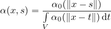
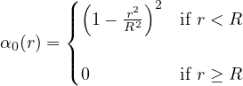
The nonlocal weight function is usually defined as

-α0-(∥x---s∥)--- α (x,s) = ∫α0(∥x - t∥)dt V

(51)

where

( || (1- r2-)2 if r < R { R2 α0(r) = || ( 0 if r ≥ R

(52)

is a nonnegative function, for r < R monotonically decreasing with increasing distance r = ∥x-s∥, and V denotes the domain occupied by the investigated material body. The key idea is that the damage evolution at a certain point depends not only on the cumulated plastic strain at that point, but also on points at distances smaller than the interaction radius R, considered as a new material parameter.

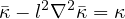
Implicit gradient formulation The gradient formulation can be conceived as the differential counterpart to the integral formulation. The nonlocal cumulated plastic strain is computed from a Helmholtz-type differential equation

2 2 ¯κ - l∇ ¯κ = κ

(53)

with homogeneous Neumann boundary condition

∂¯κ- ∂n = 0.

(54)

In (53), l is the length scale parameter and ∇ is the Laplace operator.

The model description and parameters are summarized in Tabs. 14 and 15. Note that the internal length parameter r has the meaning of the radius of interaction R for the integral version (and thus has the dimension of length) but for the gradient version it has the meaning of the coefficient l² multiplying the Laplacean in (53), and thus has the dimension of length squared.


Description	Nonlocal Mises plasticity with isotropic hardening

Record Format	MisesMatNl (in) # d(rn) # E(rn) # n(rn) # sig0(rn) # H(rn) # omega_crit(rn) #a(rn) #r(rn) #m(rn) #[wft(in) #][scalingType(in) #]
Parameters	- material number
	- d material density
	- E Young’s modulus
	- n Poisson’s ratio
	- sig0 initial yield stress in uniaxial tension (compression)
	- H hardening modulus
	- omega_crit critical damage
	- a exponent in damage law
	- r nonlocal interaction radius R from eq. (52)
	- m over-nonlocal parameter
	- wft selects the type of nonlocal weight function (see Section 1.5.7): default, quartic spline (bell-shaped function with bounded support) Gaussian function exponential function (Green function in 1D) uniform averaging up to distance R uniform averaging over one finite element special function obtained by reducing the 2D exponential function to 1D (by numerical integration)
	- scalingType selects the type of scaling of the weight function (e.g. near a boundary; see Section 1.5.7): default, standard scaling with integral of weight function in the denominator no scaling (the weight function normalized in an infinite body is used even near a boundary) Borino scaling (local complement)
Supported modes	1dMat, PlaneStrain, 3dMat

Table 14: Nonlocal integral Mises plasticity – summary.


Description	Gradient-enhanced Mises plasticity with isotropic damage

Record Format	MisesMatGrad (in) # d(rn) # E(rn) # n(rn) # sig0(rn) # H(rn) # omega_crit(rn) #a(rn) #r(rn) #m(rn) #
Parameters	- material number
	- d material density
	- E Young’s modulus
	- n Poisson’s ratio
	- sig0 initial yield stress in uniaxial tension (compression)
	- H hardening modulus
	- omega_crit critical damage
	- a exponent in damage law
	- r internal length scale parameter l² from eq. (53)
	- m over-nonlocal parameter
Supported modes	1dMat, PlaneStrain, 3dMat

Table 15: Gradient-enhanced Mises plasticity – summary.

1.4.5 Rankine plasticity model with isotropic damage and its nonlocal formulations - RankMat, RankMatNl, RankMatGrad

This model has a very similar structure to the model described in Section 1.4.3, but is based on the Rankine yield condition. It is available in the small-strain version only, and so far exclusively for plane stress analysis. The basic equations (40)–(41) and (43)–(47) remain valid, and the yield function (42) is redefined as

f (σ¯, κ) = max ¯σI - σY (κ) I

(55)

where σ_I are the principal values of the effective stress tensor σ. The hardening law can have either the linear form (44), or the exponential form

σY(κ) = σ0 +Δ σY (1 - exp(- H κ∕ΔσY )),

(56)

where H is now the initial plastic modulus and Δσ_Y is the value of yield stress increment asymptotically approached as κ →∞. In damage law (47), parameter ω_c is always set to 1. If the plastic hardening is linear, the user can specify either the exponent a from (47), or the dissipation per unit volume, g_f, which represents the area under the stress-strain diagram (and parameter a is then determined automatically such that the area under the diagram has the prescribed value). For exponential plastic hardening, the evaluation of a from g_f is not properly implemented and it is better to specify a directly.

The model description and parameters are summarized in Tabs. 16–18. Note that the default value of parameter m is equal to 1 for the integral model but for the gradient model it is equal to 2. Also note that the internal length parameter r has the meaning of the radius of interaction R for the integral version (and thus has the dimension of length) but for the gradient version it has the meaning of the coefficient l² multiplying the Laplacean in (53), and thus has the dimension of length squared.

For the gradient model it is possible to specify parameter negligible_damage, which sets the minimum value of damage that is considered as nonzero. The approximate solution of Helmholtz equation (53) can lead to very small but nonzero nonlocal kappa at some points that are actually elastic. If such small values are positive, they lead to a very small but nonzero damage. If this is interpreted as ”loading”, the tangent terms are activated, but damage will not actually grow at such points and the convergence rate is slowed down. It is better to consider such points as elastic. By default, negligible_damage is set to 0, but it is recommended to set it e.g. to 1.e-6.


Description	Rankine plasticity with isotropic hardening and damage

Record Format	RankMat (in) # d(rn) # E(rn) # n(rn) # plasthardtype(in) # sig0(rn) # H(rn) # delSigY(rn) # yieldtol(rn) # (gf(rn) # ∥ a(rn) #)
Parameters	- material number
	- d material density
	- E Young’s modulus
	- n Poisson’s ratio
	- plasthardtype type of plastic hardening (0=linear=default, 1=exponential)
	- sig0 initial yield stress in uniaxial tension (compression)
	- H initial hardening modulus (default value 0.)
	- delSigY final increment of yield stress (default value 0., needed only if plasthardtype=1)
	- yieldtol relative tolerance in the yield condition
	- gf dissipation per unit volume
	- a exponent in damage law (47)
Supported modes	PlaneStress

Table 16: Rankine plasticity – summary.


Description	Nonlocal Rankine plasticity with isotropic hardening and damage

Record Format	RankMatNl (in) # d(rn) # E(rn) # n(rn) # plasthardtype(in) # sig0(rn) # H(rn) # delSigY(rn) # yieldtol(rn) # (gf(rn) # ∥ a(rn) #)r(rn) #m(rn) #[wft(in) #][scalingType(in) #]
Parameters	- material number
	- d material density
	- E Young’s modulus
	- n Poisson’s ratio
	- plasthardtype type of plastic hardening (0=linear=default, 1=exponential)
	- sig0 initial yield stress in uniaxial tension (compression)
	- H initial hardening modulus (default value 0.)
	- delSigY final increment of yield stress (default value 0.)
	- yieldtol relative tolerance in the yield condition
	- gf dissipation per unit volume
	- a exponent in damage law (47)
	- r internal length scale parameter l² from eq. (53)
	- m over-nonlocal parameter (default value 1.)
	- wft selects the type of nonlocal weight function (see Section 1.5.7): default, quartic spline (bell-shaped function with bounded support) Gaussian function exponential function (Green function in 1D) uniform averaging up to distance R uniform averaging over one finite element special function obtained by reducing the 2D exponential function to 1D (by numerical integration)
	- scalingType selects the type of scaling of the weight function (e.g. near a boundary; see Section 1.5.7): default, standard scaling with integral of weight function in the denominator no scaling (the weight function normalized in an infinite body is used even near a boundary) Borino scaling (local complement)
Supported modes	PlaneStress

Table 17: Nonlocal integral Rankine plasticity – summary.


Description	Gradient-enhanced Rankine plasticity with isotropic hardening and damage

Record Format	RankMatGrad (in) # d(rn) # E(rn) # n(rn) # plasthardtype(in) # sig0(rn) # H(rn) # delSigY(rn) # yieldtol(rn) # (gf(rn) # ∥ a(rn) #)r(rn) #m(rn) #negligible_damage(rn) #
Parameters	- material number
	- d material density
	- E Young’s modulus
	- n Poisson’s ratio
	- plasthardtype type of plastic hardening (0=linear=default, 1=exponential)
	- sig0 initial yield stress in uniaxial tension (compression)
	- H hardening modulus (default value 0.)
	- delSigY final increment of yield stress (default value 0.)
	- yieldtol relative tolerance in the yield condition
	- gf dissipation per unit volume
	- a exponent in damage law (47)
	- r internal length scale parameter l from eq. (53)
	- m over-nonlocal parameter (default value 2.)
	- negligible_damage optional parameter (default value 0.)
Supported modes	PlaneStress

Table 18: Gradient-enhanced Rankine plasticity – summary.

1.4.6 Perfectly plastic material with Mises yield condition - Steel1

This is an older model, kept here for compatibility with previous versions. It uses Mises plasticity condition with no hardening and under small strain only. The model description and parameters are summarized in Tab. 19. All its features are included in the model described in Section 1.4.3.


Description	Perfectly plastic material with Mises condition

Record Format	Steel1 num(in) # d(rn) # E(rn) # n(rn) # tAlpha(rn) # Ry(rn) #
Parameters	- num material model number
	- d material density
	- E Young modulus
	- n Poisson ratio
	- tAlpha thermal dilatation coefficient
	- Ry uniaxial yield stress
Supported modes	3dMat, PlaneStress, PlaneStrain, 1dMat, 2dPlateLayer, 2dBeamLayer, 3dShellLayer 3dBeam, PlaneStressRot

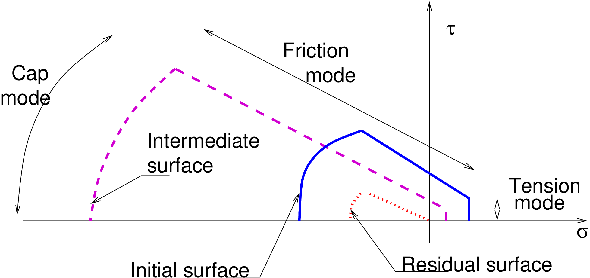
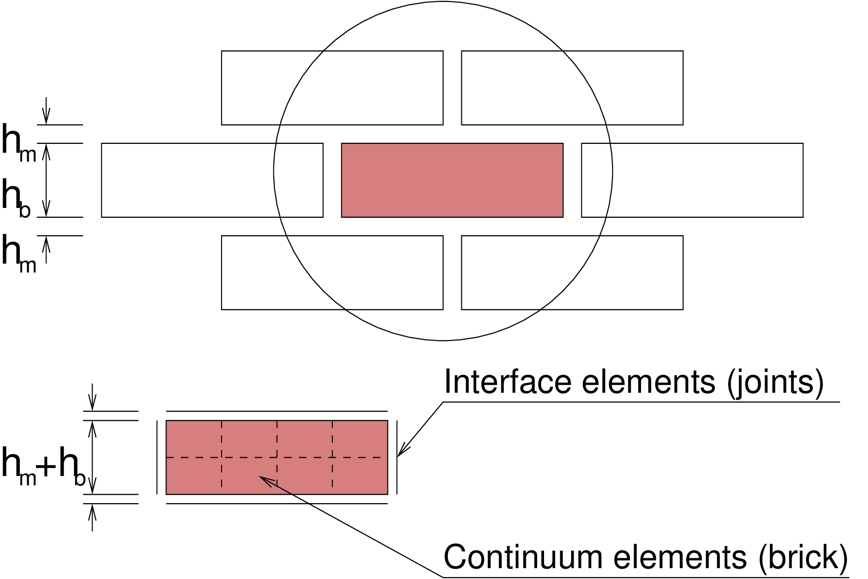
Table 19: Perfectly plastic material with Mises condition – summary.

1.4.7 Composite plasticity model for masonry - Masonry02

Masonry is a composite material made of bricks and mortar. Nonlinear behavior of both components should be considered to obtain a realistic model able to describe cracking, slip, and crushing of the material. The model is based on paper by Lourenco and Rots [18]. It is formulated on the basis of softening plasticity for tension, shear, and compression (see fig.(1)). Numerical implementation is based on modern algorithmic concepts such as implicit integration of the rate equations and consistent tangent stiffness matrices.

Figure 1: Composite yield surface model for masonry

The approach used in this work is based on idea of concentrating all the damage in the relatively weak joints and, if necessary, in potential tension cracks in the bricks. The joint interface constitutive model should include all important damage mechanisms. Here, the concept of interface elements is used. An interface element allows to incorporate discontinuities in the displacement field and its behavior is described in terms of a relation between the tractions and relative displacement across the interface. In the present work, these quantities will be denoted as σ, generalized stress, and ε, generalized strain. For 2D configuration, σ = {σ,τ}^T and ε = {u_n,u_s}^T, where σ and τ are the normal and shear components of the traction interface vector and n and s subscripts distinguish between normal and shear components of displacement vector.

Figure 2: Modeling strategy for masonry

The elastic response is characterized in terms of elastic constitutive matrix D as

σ = D ε

(57)

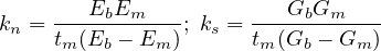
For a 2D configuration D = diag{k_n,k_s}. The terms of the elastic stiffness matrix can be obtained from the properties of both masonry and joints as

kn =---EbEm---- ; ks =---GbGm----- tm (Eb - Em ) tm (Gb - Gm )

(58)

where E_b and E_m are Young’s moduli, G_b and G_m shear moduli for brick and mortar, and t_m is the thickness of joint. One should note, that there is no contact algorithm assumed between bricks, this means that the overlap of neighboring units will be visible. On the other hand, the interface model includes a compressive cap, where the compressive inelastic behavior of masonry is lumped.

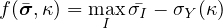
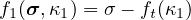
Tension mode In the tension mode, the exponential softening law is assumed (see fig.(3)). The yield function has the following form

f (σ,κ ) = σ - f(κ ) 1 1 t 1

(59)

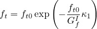
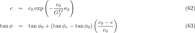
where the yield value f_t is defined as

( ) f = f exp - ft0-κ t t0 GIf 1

(60)

Figure 3: Tensile behavior of proposed model (f_t = 0.2 MPa, G_f^I = 0.018 N/mm)

The f_t0 represents tensile strength of joint or interface; and G_f^I is mode-I fracture energy. For the tension mode, the associated flow hypothesis is assumed.

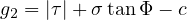
Shear mode For the shear mode a Coulomb friction envelope is used. The yield function has the form

f2(σ,κ2) = |τ|+ σtanϕ(κ2)- c(κ2)

(61)

According to [18] the variations of friction angle ϕ and cohesion c are assumed as

( ) c = c exp - c0-κ (62) 0 GIfI 2 (c - c ) tan ϕ = tanϕ0 + (tanϕr - tan ϕ0) -0--- (63) c0

where c₀ is initial cohesion of joint, ϕ₀ initial friction angle, ϕ_r residual friction angle, and G_f^II fracture energy in mode II failure. A non-associated plastic potential g₂ is considered as

g2 = |τ|+ σ tan Φ- c

(64)

Figure 4: Shear behavior of proposed model for different confinement levels in MPa (c₀ = 0.8 MPa, tanϕ₀ = 1.0, tanϕ_r = 0.75,and G_f^II = 0.05 N∕mm)

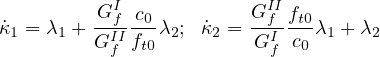
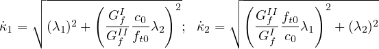
Coupling of tension/shear modes The tension and Coulomb friction modes are coupled with isotropic softening. This means that the percentage of softening in the cohesion is assumed to be the same as on the tensile strength

˙κ = λ + GIf-c0λ ; κ˙ = GIIf-ft0λ + λ 1 1 GIIf ft0 2 2 GIf c0 1 2

(65)

This follows from (60) and (62). However, in the corner region, when both yield surfaces are activated, such approach will lead to a non-acceptable penalty. For this reason a quadratic combination is assumed

┌│ -------(---------)2 ┌│ (---------)2------- │∘ 2 GIf-c0- │∘ GIfIft0 2 ˙κ1 = (λ1) + GIfIft0λ2 ; κ˙2 = GIf c0 λ1 +(λ2)

(66)

Cap mode For the cap mode, an ellipsoid interface model is used. The yield condition is assumed as

f3(σ,κ3) = Cnn σ2 + Cssτ2 + Cnσ - ¯σ2(κ3)

(67)

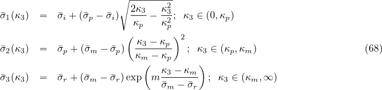
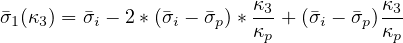
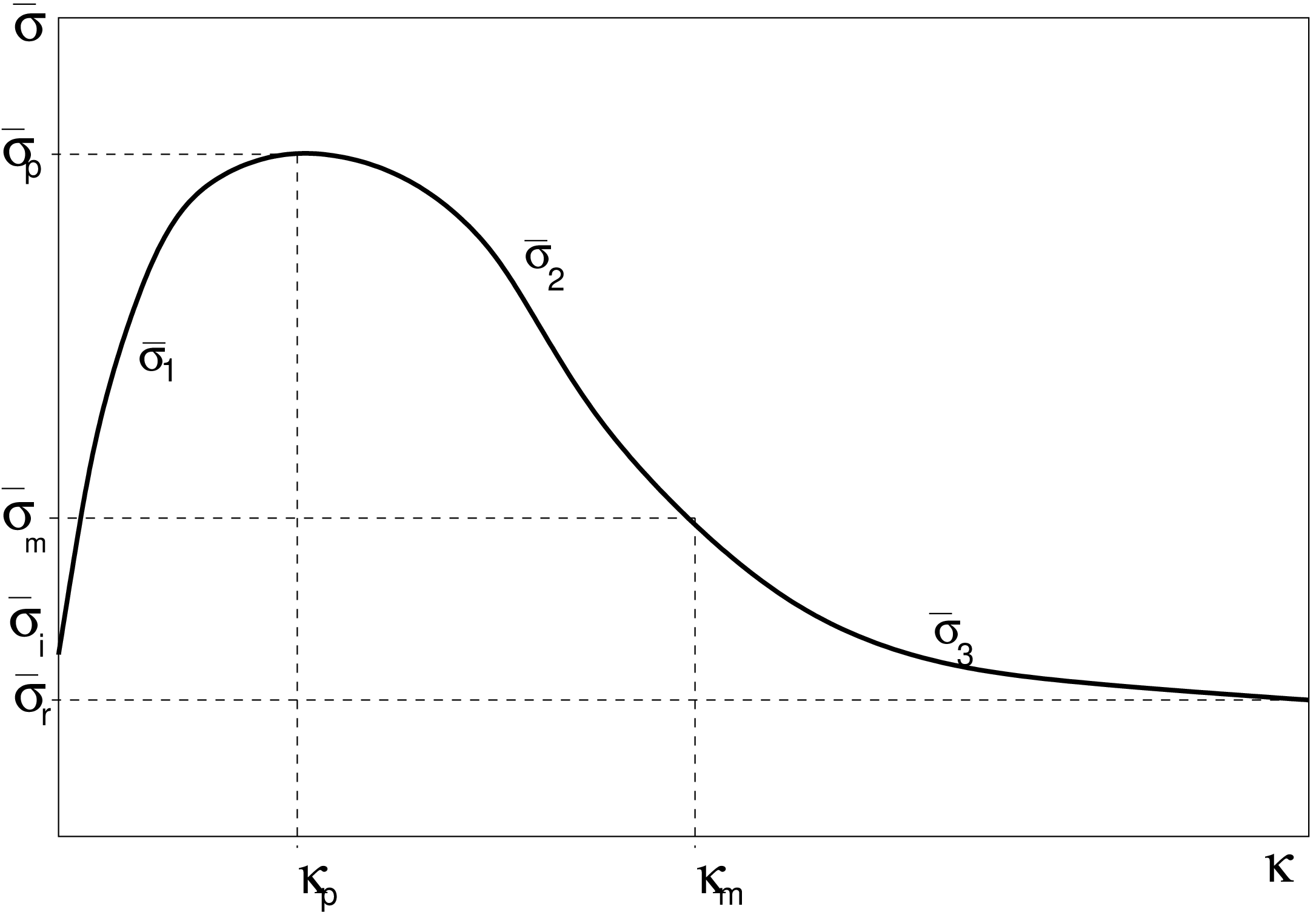
where C_nn, C_ss, and C_n are material model parameters and σ is yield value, originally assumed in the following form of hardening/softening law [18]

∘ -------2- σ¯1(κ3) = ¯σi + (¯σp - ¯σi) 2κ3- κ-3; κ3 ∈ (0,κp) κp κ2p ( κ - κ )2 σ¯2(κ3) = ¯σp + (¯σm - ¯σp) -3---p- ; κ3 ∈ (κp,κm ) (68) κm( - κp ) σ¯3(κ3) = ¯σr + (¯σm - ¯σr)exp mκ3---κm ; κ3 ∈ (κm, ∞) σ¯m - ¯σr

with m = 2(σ_m -σ_p)∕(κ_m - κ_p). The hardening/softening law (68) is shown in fig.(5). Note that the curved diagram is a C¹ continuous σ - κ₃ relation. The energy under the load-displacement diagram can be related to a “compressive fracture energy”. The original hardening law (68.1) exhibits indefinite slope for κ₃ = 0, which can cause the problems with numerical implementation. This has been overcomed by replacing this hardening law with parabolic equation given by

¯σ1(κ3) = ¯σi - 2* (σ¯i -σ¯p) * κ3 + (σ¯i - ¯σp)κ3 κp κp

(69)

An associated flow and strain hardening hypothesis are being considered. This yields

∘------------------------------------------ ˙κ3 = λ3 (2Cnn σ+ Cn) *(2Cnnσ +Cn )+ (2Cssτ)*(2Cssτ)

(70)

Figure 5: Hardening/softening law for cap mode

The model parameters are summarized in Tab. 20. There is one algorithmic issue, that follows from the model formulation. Since the cap mode hardening/softening is not coupled to hardening/softening of shear and tension modes the it may happen that when the cap and shear modes are activated, the return directions become parallel for both surfaces. This should be avoided by adjusting the input parameters accordingly (one can modify dilatancy angle, for example).


Description	Composite plasticity model for masonry

Record Format	Masonry02 num(in) # d(rn) # E(rn) # n(rn) # ft0(rn) # gfi(rn) # gfii(rn) # kn(rn) # ks(rn) # c0(rn) # tanfi0(rn) # tanfir(rn) # tanpsi(rn) # si(rn) # sp(rn) # sm(rn) # sr(rn) # kp(rn) # km(rn) # kr(rn) # cnn(rn) # css(rn) # cn(rn) #
Parameters	- num material model number
	- d material density
	- E Young modulus
	- n Poisson ratio
	- ft0 tensile strength
	- gfi fracture energy for mode I
	- gfii fracture energy for mode II
	- kn joint elastic property
	- ks joint elastic property
	- c0 initial cohesion
	- tanfi0 initial friction angle
	- tanfir residual friction angle
	- tanpsi dilatancy
	- {si, sp, sm, sr} cap parameters {σ_i,σ_p,σ_m,σ_r}
	- {kp, km,kr} cap parameters {κ_p,κ_m,κ_r}
	- cnn,css,cn cap mode parametrs
Supported modes	_2dInterface

Table 20: Composite model for masonry - summary.

1.4.8 Nonlinear elasto-plastic material model for concrete plates and shells - Concrete2

Nonlinear elasto-plastic material model with hardening. Takes into account uniaxial stress + transverse shear in concrete layers with transverse stirrups. Can be used only for 2d plates and shells with layered cross section and together with explicit integration method (stiffness matrix is not provided). The model description and parameters are summarized in Tab. 21.


Description	Nonlinear elasto-plastic material model for concrete plates and shells

Record Format	Concrete2 num(in) # d(rn) # E(rn) # n(rn) # SCCC(rn) # SCCT(rn) # EPP(rn) # EPU(rn) # EOPU(rn) # EOPP(rn) # SHEARTOL(rn) # IS_PLASTIC_FLOW(in) # IFAD(in) # STIRR_E(rn) # STIRR_Ft(rn) # STIRR_A(rn) # STIRR_TOL(rn) # STIRR_EREF(rn) # STIRR_LAMBDA(rn) #
Parameters	- num material model number
	- d material density
	- E Young modulus
	- n Poisson ratio
	- SCCC pressure strength
	- SCCT tension strength
	- EPP threshold effective plastic strain for softening in compression
	- EPU ultimate eff. plastic strain
	- EOPP threshold volumetric plastic strain for softening in tension
	- EOPU ultimate volumetric plastic strain
	- SHEARTOL threshold value of the relative shear deformation (psi**2/eef) at which shear is considered in layers. For lower relative shear deformations the transverse shear remains elastic decoupled from bending. default value SHEARTOL = 0.01
	- IS_PLASTIC_FLOW indicates that plastic flow (not deformation theory) is used in pressure
	- IFAD State variables will not be updated, otherwise update state variables
	- STIRR_E Young modulus of stirrups
	- STIRR_R stirrups uniaxial strength = elastic limit
	- STIRR_A stirrups area/unit length (beam) or /unit area (shell)
	- STIRR_TOL stirrups tolerance of equilibrium in the z direction (=0 no iteration)
	- STIRR_EREF stirrups reference strain rate for Peryzna’s material
	- STIRR_LAMBDA coefficient for that material (stirrups)
	- SHTIRR_H isotropic hardening factor for stirrups
Supported modes	3dShellLayer, 2dPlateLayer

Table 21: Nonlinear elasto-plastic material model for concrete - summary.

[next] [prev] [prev-tail] [front] [up]