Non-stationary linear transport model
The weak form of diffusion-type differential equation leads to
where the matrix
is a general non-symmetric conductivity matrix,
is a general capacity matrix and the vector
contains contributions from external and internal sources. The vector of unknowns,
, can hold nodal values of temperature, humidity, or concentration fields, for example.
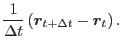
Time discretization is based on a generalized trapezoidal rule. Let us assume that the solution is known at time
and the time increment is
. The parameter
defines a type of integration scheme;
results in an explicit (forward) method,
refers to the Crank-Nicolson method, and
means an implicit (backward) method. The appromation of solution vector and its time derivative yield
![$\displaystyle \tau$](img249.png) |
![$\displaystyle =$](img51.png) |
![$\displaystyle t+\alpha\Delta t = (t+\Delta t) - (1-\alpha)\Delta t,$](img250.png) |
(2.9) |
![$\displaystyle \mbox{\boldmath$r$}$](img126.png) ![$\displaystyle _{\tau}$](img251.png) |
![$\displaystyle =$](img51.png) |
![$\displaystyle (1-\alpha)$](img252.png) ![$\displaystyle \mbox{\boldmath$r$}$](img126.png) ![$\displaystyle _t+\alpha$](img253.png) ![$\displaystyle \mbox{\boldmath$r$}$](img126.png) ![$\displaystyle _{t+\Delta t},$](img254.png) |
(2.10) |
![$\displaystyle \frac{{\rm d}\mbox{\boldmath$r$}}{{\rm d} t}$](img255.png) |
![$\displaystyle =$](img51.png) |
![$\displaystyle \frac{1}{\Delta t}\left(\mbox{\boldmath$r$}_{t+\Delta t}-\mbox{\boldmath$r$}_t\right).$](img256.png) |
(2.11) |
![$\displaystyle \mbox{\boldmath$F$}$](img107.png) ![$\displaystyle _{\tau}$](img251.png) |
![$\displaystyle =$](img51.png) |
![$\displaystyle (1-\alpha)$](img252.png) ![$\displaystyle \mbox{\boldmath$F$}$](img107.png) ![$\displaystyle _t+\alpha$](img253.png) ![$\displaystyle \mbox{\boldmath$F$}$](img107.png) ![$\displaystyle _{t+\Delta t},$](img254.png) |
(2.12) |
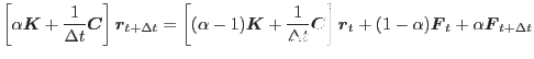
Let us assume that Eq. (2.8) should be satisfied at time
. Inserting
into Eq. (2.8) leads to
![$\displaystyle \left[\alpha \mbox{\boldmath$K$} + \frac{1}{\Delta t} \mbox{\bold...
... +
(1-\alpha) \mbox{\boldmath$F$}_{t} + \alpha \mbox{\boldmath$F$}_{t+\Delta t}$](img258.png) |
|
|
(2.13) |
where the conductivity matrix
contains also a contribution from convection, since it depends on
![$ r$](img5.png)
The vectors
![$ F$](img100.png)
or
![$ F$](img100.png)
contain all known contributions
![$\displaystyle \mbox{\boldmath$F$}$](img107.png) ![$\displaystyle _t = - \underbrace{\int_{\Gamma_{\overline{q}}} \mbox{\boldmath$N...
..._{\Omega}\mbox{\boldmath$N$}^T\overline{Q}_t\mathrm{d}\Omega}_{\textrm{Source}}$](img264.png) |
|
|
(2.15) |
Borek Patzak
2017-12-30