We start by assuming the parametrized loading, in which the total external load vector is expressed as
where

 is proportional, reference load vector, and
  is load scaling parameter,
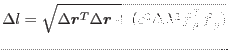
The arc-length method is based on idea of controlling the length passed along the loading path. For the differential length of loading path we can write
is load scaling parameter,
The arc-length method is based on idea of controlling the length passed along the loading path. For the differential length of loading path we can write
 |
(2.3) |
where  is coefficient of generalized metrics used to define
  (taking into account different units of displacement and load).
For selected increment of loading path length , we are looking for the equilibrium, where the unknowns are nodal displacements
(taking into account different units of displacement and load).
For selected increment of loading path length , we are looking for the equilibrium, where the unknowns are nodal displacements
 and the load scaling parameter . We have the equilibrium equation and additional scalar equation 2.3:
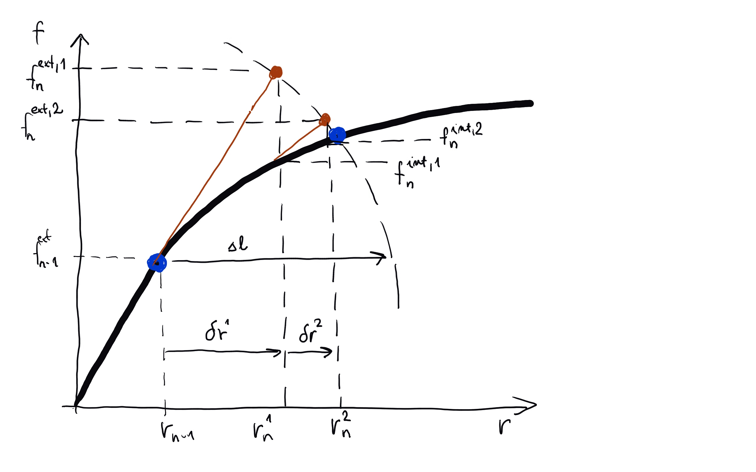
Figure 2.2:
Illustration of Acr-length method
|
|
At the end of n-th loading step and i-th iteration the displacement vector can be written as

 and similarly the load scaling parameter as
 . Substituting this into equilibrium equation 2.4 we get
By linearization of

 around known state
 we get
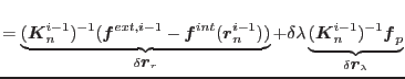
and finally for unknown

Note that the vectors
 and
and
 can be computed and the only unknown remaining is the incremental change of loading parameter
 , which could be determined from 2.5
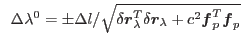
This finally yields a quadratic equation for unknown increment of loading parameter
. The algorithm is summarized in Table ![[*]](crossref.png) .
.
Table 2.2:
Newton-Raphson method
| Given |
|
 |
|
  |
|
| Evaluate |
|
    |
|
 |
|
       |
|
Repeat for
 |
|
 |
|
    |
|
 Solve quadratic equation 2.7 for Solve quadratic equation 2.7 for
|
|
  |
|
      |
|
 |
|
| Until convergence reached |
|
|
Borek Patzak
2017-12-30