Linear isotropic material model. The model parameters are summarized in Tab. 1.
| Description | Linear isotropic elastic material |
| Record Format | IsoLE num(in) # d(rn) # E(rn) # n(rn) # tAlpha(rn) # |
| Parameters | - num material model number |
| - d material density | |
| - E Young modulus | |
| - n Poisson ratio |
|
| - tAlpha thermal dilatation coefficient |
|
| Supported modes | 3dMat, PlaneStress, PlaneStrain, 1dMat, 2dPlateLayer, 2dBeamLayer, 3dShellLayer, 2dPlate, 2dBeam, 3dShell, 3dBeam, PlaneStressRot |
| Features | Adaptivity support |
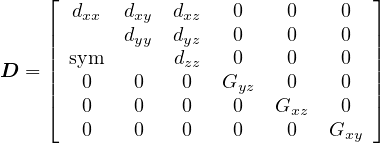
Orthotropic, linear elastic material model. The model parameters are summarized in Tab. 2. Local coordinate system, which determines axes of material orthotrophy can by specified using lcs array. This array contains six numbers, where the first three numbers represent directional vector of a local x-axis, and next three numbers represent directional vector of a local y-axis. The local z-axis is determined using the vector product. The right-hand coordinate system is assumed.
Local coordinate system can also be specified using scs parameter. Then local coordinate system is specified in so called “shell” coordinate system, which is defined locally on each particular element and its definition is as follows: principal z-axis is perpendicular to shell mid-section, x-axis is perpendicular to z-axis and normal to user specified vector (so x-axis is parallel to plane, with being normal to this plane) and y-axis is perpendicular both to x and z axes. This definition of coordinate system can be used only with plates and shells elements. When vector is parallel to z-axis an error occurs. The scs array contain three numbers defining direction vector . If no local coordinate system is specified, by default a global coordinate system is used.
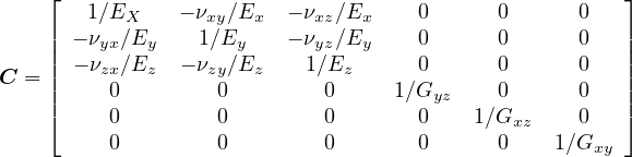
For 3D case the material compliance matrix has the following form
| (1) |
By inversion, the material stiffness matrix has the form
| (2) |
where ξ = 1 - (νxy * νyx + νyz * νzy + νzx * νxz) - (νxy * νyz * νzx + νyx * νzy * νxz) and
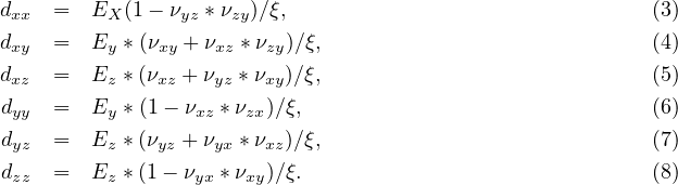
Ei is Young’s modulus in the i-th direction, Gij is the shear modulus in ij plane, νij is the major Poisson ratio, and νji is the minor Poisson ratio. Assuming that Ex > Ey > Ez, νxy > νyx etc., then νxy is referred to as the major Poisson ratio, while νyx is referred as the minor Poisson ratio. Note that there are only nine independent material parameters, because of symmetry conditions. The symmetry condition yields

The model description and parameters are summarized in Tab. 2.
| Description | Orthotropic, linear elastic material |
| Record Format | OrthoLE num(in) # d(rn) # Ex(rn) # Ey(rn) # Ez(rn) # NYyz(rn) # NYxz(rn) # NYxy(rn) # Gyz(rn) # Gxz(rn) # Gxy(rn) # tAlphax(rn) # tAlphay(rn) # tAlphaz(rn) # [ lcs(ra) #] [ scs(ra) #] |
| Parameters | - num material model number |
| - d material density | |
| - Ex, Ey, Ez Young moduli for x,y, and z directions | |
| - NYyz, NYxz, NYxy major Poisson’s ratio coefficients | |
| - Gyz, Gxz, Gxy shear moduli | |
| - tAlphax, tAlphay, tAlphaz thermal dilatation coefficients in x,y,z directions |
|
| - lcs Array defining local material x and y axes of orthotrophy |
|
| - scs Array defining a normal vector n. The local x axis is parallel to plane with n being plane normal. The material local z-axis is perpendicular to shell mid-section. |
|
| Supported modes | 3dMat, PlaneStress, PlaneStrain, 1dMat, 2dPlateLayer, 2dBeamLayer, 3dShellLayer, 2dPlate, 2dBeam, 3dShell, 3dBeam, PlaneStressRot |
Linear elastic material model with completely general material stiffness (21 independent elastic constants). The model parameters are summarized in Tab. 3. The material stiffness matrix is a completely arbitrary symmetric 6 × 6 matrix. The input line must contain an array with the upper triangle of this matrix. This array has length 21 and the stiffness coefficients are listed in each row from the diagonal to the last column.
| Description | Anisotropic, linear elastic material |
| Record Format | OrthoLE num(in) # d(rn) # stiff(ra) # tAlphax(ra) # |
| Parameters | - num material model number |
| - d material density | |
| - stiff real array of length 21 with stiffness coefficients D11, D12, D13…D66 |
|
| - tAlpha real array of length 0 or 3 with thermal dilatation coefficients in x,y,z directions |
|
| Supported modes | 3dMat, PlaneStress, PlaneStrain, 1dMat |
Bi-linear material model for 1D elasticity, with different elastic moduli in tension and compression. The model parameters are summarized in Tab. 4.
| Description | Bi-Linear elastic material |
| Record Format | IsoAxysymm1D num(in) # d(rn) # Et(rn) # Ec(rn) # tAlpha(rn) # [m(rn) #] |
| Parameters | - num material model number |
| - d material density | |
| - Et Modulus of elasticity in tension |
|
| - Ec Modulus of elasticity in compression |
|
| - tAlpha thermal dilatation coefficient |
|
| - m optional regularization coefficient, default value set to 15, higher value makes response close to trully bilinear |
|
| Supported modes | 1dMat |
| Features | Adaptivity support |
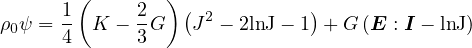
This material model can describe elastic behavior at large strains. A hyperelastic model postulates the existence of free energy potential. Existence of the potential implies reversibility of deformations and no energy dissipation during loading process. Here we use the free energy function introduced in [21]
| (9) |
where K is the bulk modulus, G is the shear modulus, J is the Jacobian (determinant of the deformation gradient, corresponding to the ratio of the current and initial volume) and E is the Green-Lagrange strain. Then stress-strain law can be derived from (9) as
| (10) |
where S is the second Piola-Kirchhoff stress, E is the Green-Lagrange strain and C is the right Cauchy-Green tensor. The model description and parameters are summarized in Tab. 5.
| Description | Hyperelastic material |
| Record Format | SimoPisterMat (in) # d(rn) # K(rn) # G(rn) # |
| Parameters | - material number |
| - d material density |
|
| - K bulk modulus |
|
| - G shear modulus |
|
| Supported modes | 3dMat |
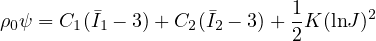
The Mooney-Rivlin strain energy function is expressed by
| (11) |
where C1 and C2 are material constants, K is the bulk modulus, J is the Jacobian (determinant of the deformation
gradient, corresponding to the ratio of the current and initial volume), 1 = J- I1, 2 = J-
 I2, where I1 and I2 are
the first and the second principal invariants of the right Cauchy-Green deformation tensor C. Compressible
neo-Hookean material model is obtained by setting C2 = 0. Then stress-strain law can be derived from (11)
as
I2, where I1 and I2 are
the first and the second principal invariants of the right Cauchy-Green deformation tensor C. Compressible
neo-Hookean material model is obtained by setting C2 = 0. Then stress-strain law can be derived from (11)
as
| (12) |
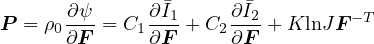
where P is the first Piola-Kirchhoff stress,
| (13) |
and
| (14) |
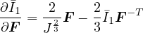
The first elasticity tensor is derived as
| (15) |
where
| (16) |
and
![4 [ 4 8 4
A2ijkl = 2J-3 I1δikδjl + 2FijFkl --I1FijF -lk1-- I2Fj-i1F-l1k - -I1F-j1i Fkl
3 9 3 ]
+4FknCnlF -1+ 2I2F -1F- 1+ 4F -1FimCmj - δikClj - FilFkj + FkmFimδjl (17)
3 ji 3 li jk 3 kl](matlibmanual14x.png)
The model description and parameters are summarized in Tab. 6.
| Description | Mooney-Rivlin |
| Record Format | MooneyRivlinCompressibleMat (in) # d(rn) # K(rn) # C1(rn) # C2(rn) # |
| Parameters | - material number |
| - d material density |
|
| - K bulk modulus |
|
| - C1 material constant |
|
| - C2 material constant |
|
| Supported modes | 3dMat, PlaneStrain |
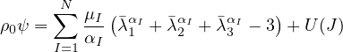
The Ogden strain energy function is expressed by
| (18) |
where μI and αI are material constants, U(J) is the volumetric part of energy, J is the Jacobian (determinant of the
deformation gradient, corresponding to the ratio of the current and initial volume), i = J- λi are the deviatoric
stretches.
λi are the deviatoric
stretches.
The model description and parameters are summarized in Tab. 7.
| Description | Ogden material |
| Record Format | OgdenCompressibleMat (in) # d(rn) # K(rn) # alpha(ra) # mu(ra) # |
| Parameters | - material number |
| - d material density |
|
| - K bulk modulus |
|
| - alpha array of material constants |
|
| - mu array of material constants |
|
| alpha and mu have to have the same size | |
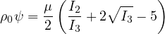
The Mooney-Rivlin strain energy function is expressed by
| (19) |
where μ is initial shear modulus, I2 and I3 are the second and third invariants of the Cauchy-Green tensor C.
The model description and parameters are summarized in Tab. 8.
| Description | Blatz-Ko material |
| Record Format | blatzkomat (in) # d(rn) # mu(rn) # |
| Parameters | - material number |
| - d material density |
|
| - mu shear modulus |
|
| ν is fixed to 0.25 | |

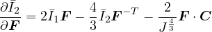

![2 2[ 2 ]
A1ijkl = 3J -3 3δikδjl + I1F-j1k F -li1- 2Fl-k1Fij + 3I1F-j1i Fl-k1- 2Fj-i1Fkl](matlibmanual13x.png)